Exporting Coordinates and Static Views

Exporting Results¶

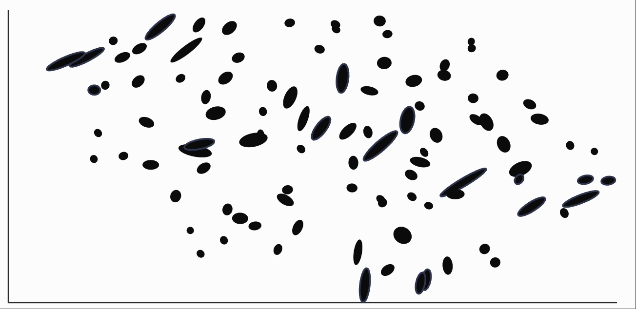
Let's first save the results from our homepage's quickstart into a plot object.

In [1]:

from distortions.geometry import Geometry, bind_metric, local_distortions, neighborhoods
from distortions.visualization import dplot
import anndata as ad
import numpy as np
import scanpy as sc

adata = ad.AnnData(np.random.poisson(2, size=(100, 5)))
sc.pp.neighbors(adata, n_neighbors=15)
sc.tl.umap(adata)

geom = Geometry(affinity_kwds={"radius": 2}, adjacency_kwds={"n_neighbors": 15})
_, Hvv, Hs = local_distortions(adata.obsm["X_umap"], adata.X, geom)
embedding = bind_metric(adata.obsm["X_umap"], Hvv, Hs)

N = neighborhoods(adata, outlier_factor=1)
plot = dplot(embedding)\
    .mapping(x="embedding_0", y="embedding_1")\
    .geom_ellipse()\
    .inter_edge_link(N=N)

from distortions.geometry import Geometry, bind_metric, local_distortions, neighborhoods from distortions.visualization import dplot import anndata as ad import numpy as np import scanpy as sc adata = ad.AnnData(np.random.poisson(2, size=(100, 5))) sc.pp.neighbors(adata, n_neighbors=15) sc.tl.umap(adata) geom = Geometry(affinity_kwds={"radius": 2}, adjacency_kwds={"n_neighbors": 15}) _, Hvv, Hs = local_distortions(adata.obsm["X_umap"], adata.X, geom) embedding = bind_metric(adata.obsm["X_umap"], Hvv, Hs) N = neighborhoods(adata, outlier_factor=1) plot = dplot(embedding)\ .mapping(x="embedding_0", y="embedding_1")\ .geom_ellipse()\ .inter_edge_link(N=N)

If you print plot, you will see the figure. Hovering the mouse near a point highlights its neighbors. If you double click the figure, it freezes the interactivity.

In [2]:

plot

plot

Out[2]:

dplot(dataset=[{'embedding_0': 1.8964743614196777, 'embedding_1': 6.912336349487305, 'x0': -0.9308546541387726…

To save a specific view, call the save() method on the plot object. By default, it will save a file plot.svg to the current notebook directory. You can specify your own path, but it must be an SVG file.

In [3]:

plot.save("output.svg")

plot.save("output.svg")

One known limitation is that you have to at least hover over the SVG before the plot will properly save. This is because anywidget loads some utilities lazily, and we can't save until some interactions have been made. The first time you run plot.save() (before any interactions), it might save an empty svg file to the directory.

In [4]:

embedding = adata.obsm["X_umap"].copy()
radius = 3 * np.mean(adata.obsp["distances"].data)
geom = Geometry("brute", laplacian_method="geometric", laplacian_kwds={"scaling_epps": 5}, adjacency_kwds={"n_neighbors": 15}, affinity_kwds={"radius": radius})
H, _, _ = local_distortions(embedding, adata.X, geom)
metrics = {k: H[k] for k in range(len(H))}
embedding = bind_metric(embedding, Hvv, Hs)

plot = dplot(embedding)\
    .mapping(x="embedding_0", y="embedding_1")\
    .inter_isometry(metrics=metrics)\
    .geom_ellipse()
plot

embedding = adata.obsm["X_umap"].copy() radius = 3 * np.mean(adata.obsp["distances"].data) geom = Geometry("brute", laplacian_method="geometric", laplacian_kwds={"scaling_epps": 5}, adjacency_kwds={"n_neighbors": 15}, affinity_kwds={"radius": radius}) H, _, _ = local_distortions(embedding, adata.X, geom) metrics = {k: H[k] for k in range(len(H))} embedding = bind_metric(embedding, Hvv, Hs) plot = dplot(embedding)\ .mapping(x="embedding_0", y="embedding_1")\ .inter_isometry(metrics=metrics)\ .geom_ellipse() plot

Out[4]:

dplot(dataset=[{'embedding_0': 1.8964743614196777, 'embedding_1': 6.912336349487305, 'x0': -0.9308546541387726…

In some cases, we don't need to save the visualization but do want to extract the coordinates after local correction. In this case, we can run the .correct() method on the plot object. If you interact with the scatterplot, freeze the view (escape or double click), and then rerun .correct(), you will see a new DataFrame giving the coordinates of the updated ellipses in the embedding_0 and embedding_1 columns. The new ellipse axes lengths and orientations are given by the remaining columns s0, ..., y0. The kernel columns provide the relatively distance between the mouse position and each sample.

In [6]:

plot.correct()

plot.correct()

Out[6]:

	embedding_0	embedding_1	s0	s1	x0	y0	new_angle	kernel_transform	kernel_metric	_id
0	1.899377	6.913011	1.142564	0.285645	-0.930853	0.365179	68.579625	0.000282	1.792812e-18	0
1	-0.567146	4.700070	0.666126	0.311308	-0.947137	-0.320688	108.705412	0.001140	1.927756e-15	1
2	-1.630083	10.627788	0.389235	0.165452	-0.997059	-0.076564	94.391133	0.003166	3.178902e-13	2
3	-0.728297	9.752711	0.560179	0.151227	-0.999498	-0.031684	91.815664	0.008311	3.964404e-11	3
4	1.550257	6.091001	0.150849	0.082332	-0.861548	-0.507579	120.504365	0.000331	3.979813e-18	4
...	...	...	...	...	...	...	...	...	...	...
95	-2.670258	9.434317	1.172215	0.463518	-0.933588	0.331331	70.460167	0.035723	5.817782e-08	95
96	-1.181273	5.239138	0.074125	0.017140	-0.789611	0.607850	52.410579	0.005154	3.638581e-12	96
97	-2.236458	6.291051	1.908003	0.464425	-0.828223	-0.517880	122.017334	0.065323	1.189392e-06	97
98	2.003829	9.243458	0.843995	0.151301	-0.994466	-0.105040	96.029506	0.000161	1.081552e-19	98
99	0.276061	9.448493	0.567533	0.407716	0.517110	0.849816	148.679624	0.003002	2.439335e-13	99

100 rows × 10 columns

In [ ]: