Teaching attention, part 2 / N: In which I don't even talk about attention
It’s a little cliche to start a post by saying that a certain type of data (in this case, sequential data) are everywhere. There’s a risk of being vague, and writing things that will become outdated, like the phrase, “soviet cybernetics”.
But sequential data are everywhere, and they are here to stay. The words in this sentence are sequential data. The order of bus stops you took to get here are sequential data. They are everywhere in society – the current capacity of water reservoirs, the cost of rice, the reach of an influenza outbreak. They are also everywhere in science – the trajectory of high energy particles at the LHC, and the sequence of biological reactions that allow cells to divide. The history of the top trending animal videos on youtube are sequential data1.
Even data that are not inherently sequential are often reformulated to be so: large images or databases can be processed one piece at a time.
These data are complicated because everything is related to everything, even if only weakly. A lot of hte videos trending from last week are still popular.
This interconnectedness makes things harder to manage, because you can’t just discard a datapoint once you’ve seen it, which is more or less what we do in settings where we claim the data are i.i.d2. A the same time, trying to keep track of everything is untenable – you would become overloaded very quickly.
What we need is a way to summarize and store everything that is important, as it arrives. We also need a way of revisiting relevant information on an as-needed basis. In the deep learning literature, these two processes are implemented through mechanisms for memory and attention.
RNNs, Revisited
Before answering such lofty questions, we will need to have a foundation in the basics3. We begin with the humblest of sequential data proceses, the recurrent neural network (RNN) cell,
\[\begin{align} h_t &= f_{\theta}\left(x_t, h_{t - 1}\right). \end{align}\]\(x_t\) are your raw input data at the \(t^{th}\) position in your sequence (“time \(t\)”). Think of \(h_{t}\) as a running summary of everything you’ve seen so far. Concretely, the input and summary data are just vectors: \(x_t \in \mathbb{R}^{n}, h_{t} \in \mathbb{R}^{k}\). The vectors are related by the function \(f_{\theta}\), parameterized by \(\theta\), which updates the current summary based on new data \(x_t\).
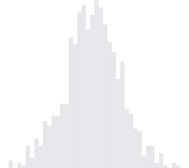
For example, let’s say that in our summary, we only care about the number of times our time series enters the interval \(\left[0, 1\right]\). Our series should look like this:
This can be easily implemented according by choosing a function \(f_{\theta}\) appropriately4,
\[\begin{align} h_{t + 1} = f_{\theta}\left(x_{t + 1}, h_t\right) := \begin{pmatrix} \mathbb{1}\{x_{t + 1} \in \left[0, 1\right]\} \\ h_{t,2} + \mathbb{1}\{h_{t, 1} = 0 \text{ and } x_{t + 1} \in \left[0, 1\right]\} \end{pmatrix} \end{align}.\]The two coordinates of \(h_t\) encode two features. The first checks whether \(x_t\) is in $\left[0, 1\right]$. The second coordinate checks whether we’re in this range, and if and if at the previous step we weren’t, then it increments its value, because an entrance has just occurred.
This is maybe one of the simplest examples of a system with memory. It takes a complicated stream of input, and carefully records the number of \(\left[0, 1\right]\) entrances. If you task at the end of each sequence were to report this count, then you can call it a day, this processor $f_{\theta}$ solves that problem entirely.
Okay it’s not that actually that simple
The general definition \(f_{\theta}\) I’ve given is a technically correct one, but in our formulation of a counter, we’ve committed a grave sin of deep learning: we have hard-coded our features. We looked at the problem, declared that the number of \(\left[0, 1\right]\) entrances was what really mattered, and hand-engineered the necessary processing unit.
In the real-world, this usually won’t be possible. Consider the problem of sentiment analysis – you’re trying to tell whether a movie review is positive or negative. No one’s going to debate that the number of occurrences of “fantastic” and “this movie is honestly the worst movie I’ve ever seen” are probably very good predictors, but it would be foolish to try to engineer all possibly predictive features by hand.
Enter, Deep Learning
To resolve this, we appeal to one of the central tenets of deep learning,
By composing simple differentiable units, we can learn useful features automatically.
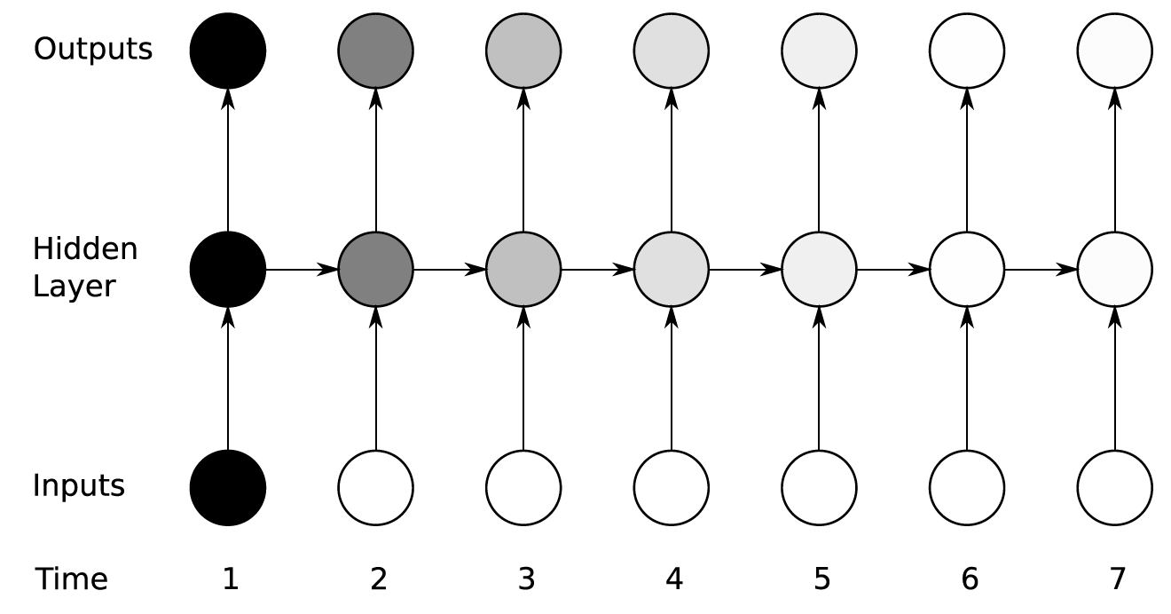
Graphically, we shift our perspective from chains of RNN cells,
where \(f_{\theta}\) might be a complex hand-engineered function, to chains and layers of simpler processing units.
The left-to-right arrows are still used to build a type of temporal memory, but now we have bottom-up function composition arrows, which help in learning complex features from otherwise simple units. A common “atom” from which these sheets are defined is the function,
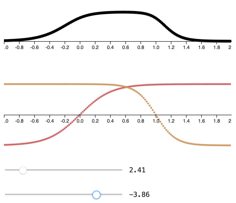
\[\begin{align} h_{t} &= \tanh\left(W_{x}x_{t} + W_{h}h_{t - 1} + b\right) \end{align}\]which has the form \(f_{\theta}\left(x_t, h_t - 1\right)\) where \(\theta = \{W_{x}, W_{h}, b\}\). It’s admittedly a relatively restricted class of functions. Through \(W_{x}\) and \(W_{h}\), it can tell whether certain linear mixtures of components of \(x_{t}\) or \(h_{t}\) are large or small, but in the end it can only return monotone functions of this mixtures, and restricted to \(\left[-1, 1\right]\) at that. That makes things sound more abstract than they really are – you can actually visualize the entire family of functions in the case that the input and summary are both two-dimensional,
These are simple, but by stacking them, we can achieve complexity, just like how stacks of ReLU units can become complicated feature detectors in computer vision. In fact, we can almost recover our \(\left[0, 1\right]\) entrance counter just by stacking a few of these units.
Define the first layer by,
\[\begin{align} h^{1}_{t} &= \tanh\left(\begin{pmatrix} + \\ - \end{pmatrix}x + \begin{pmatrix} 0 \\ -\end{pmatrix}\right) \end{align}\]so that the first coordinate tells us if we’re larger than 0, and the second tells us if we’re less than 1. Here, \(+\) and \(-\) are arbitrary positive and negative values, respectively.
In the second layer, we combine these two pieces of information, to see if we’re in the \(\left[0, 1\right]\) range,
\[\begin{align} h_{t}^{2} &= \tanh(1^{T} h_{t}^{1}). \end{align}\]These two units are visualized in the interactive figure linked below.
In the last, we need to introduce a sense of history,
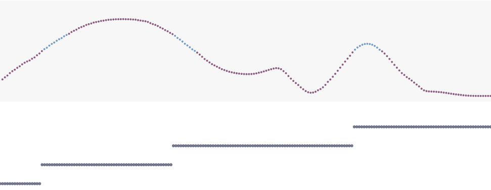
\[\begin{align} h_{t}^{3} &= \tanh\left(w_{1} h_{t - 1}^{3} + w_{2} h_{t}^{2}\right) \end{align}\]Remember, we want to build a counter, but only have access to \(\tanh\)-like units, which are bounded5. The here is to use the first term, \(w_{1}{h_{t - 1}^{3}}\) to maintain a memory of the current counter state, while the second, \(w_{2}{h_{t}^{2}}\) adds to the counter whenever it detects that we have made a \(\left[0, 1\right]\) entrance.
The figure below shows that this more or less works, but that there is a tradeoff. Making \(w_{1} \gg w_{2}\) means that increments to the count are hard to notice, but they are retained in memory for a long time. On the other hand, when \(w_1 << w_2\), we can easily see when we’ve entered the state, but there is a risk that the counter “forgets” what it’s earlier value was.
Gating and Memory
What we’re noticing is an instance of the “vanishing gradient” problem, which is elegantly illustrated by Figure 4.16 from Graves’ Sequence Labeling book,
There is a remarkably simple solution to this problem: gating. The idea is that if the value of a feature at a particular point is potentially important for something later on, we block off any updates to it that would otherwise be made by all the incoming data. This process of blocking off updates is called “gating”. It’s like we decide the current value is important, and we place it under a glass case, where it is untouched by anything else in the world. At any point, it’s value can be read, but not changed.
If at some future point, we decide we need to change the feature’s value, we take it out of the case. We ungate what had been a gated value.
How do you actually implement something like this? In principle, you could define a binary value for each feature coordinate, demarcating whether the value can be changed at the current timestep. Then, you could try to learn a good pattern of 0s and 1s from training examples – you might realize that certain types of input are useful in the long run, and should always be gated.
In practice, learning binary patterns is difficult, since such a mask wouldn’t be differentiable. Instead, we use sigmoid units, which are smooth surrogates that achieve the same effect. If you pursue this line of thinking for long enough, you woudl probably arrive at something similar (if not identical) to LSTM or GRUs7.
Mechanics of GRUs
A GRU is defined by the update,
\[\begin{align} h_t &= \left(1 - z_t\right)h_{t - 1} + z_{t}\tilde{h}_{t} \end{align}\]which interpolates between the previous state and some new candidate, according to some factor \(z_{t}\). To make \(z_{t}\) learnable, it’s set to a sigmoid over inputs and states,
\[\begin{align} z_t &= \sigma\left(W_z x_t + U_z h_{t - 1}\right) \end{align}\]The candidate is tricker, because it has a notion of a reset \(r_{t}\),
\[\begin{align} \tilde{h}_{t} &= \tanh\left(Wx_t + U\left(r_t \circ h_{t - 1}\right)\right) \end{align}\]I think of \(z_t\) as a kind of hesitant forgetting: overwriting you have to do in order to write anything new to \(h_t\), while \(r_t\) is a brutal “deliberate” forgetting, which wasn’t strictly necessary.
Note that to adapt the toy counter, it’s only necessary to introduce gatings through \(z_t\)’s.
Finally, a real example
To be honest, I didn’t want to spend so much time on gated RNNs. However,
- So many of the diagrams explaining these ideas are so complicated (at least to me, I mean, as useful as they are, does any get geometric intuition from computational graphs?), that I couldn’t just copy and paste8.
- Gating is central to understanding memory and attention. All the other mechanisms discussed in this series are variants of the basic recipe of knowing what to write as features for long-term reference and having clear ways to access them when needed.
I’m also a little tired of coming up with all these weights by hand – don’t take your optimizers for granted!
Exercise: Train a gated RNN to perform the \(\left[0, 1\right]\) entrance counting task, starting from a random initialization. How does the number of layers / number of units in each layer affect the ease of training? How does that relate to what we know about being able to hand-craft an RNN that solves the task using only very few units.
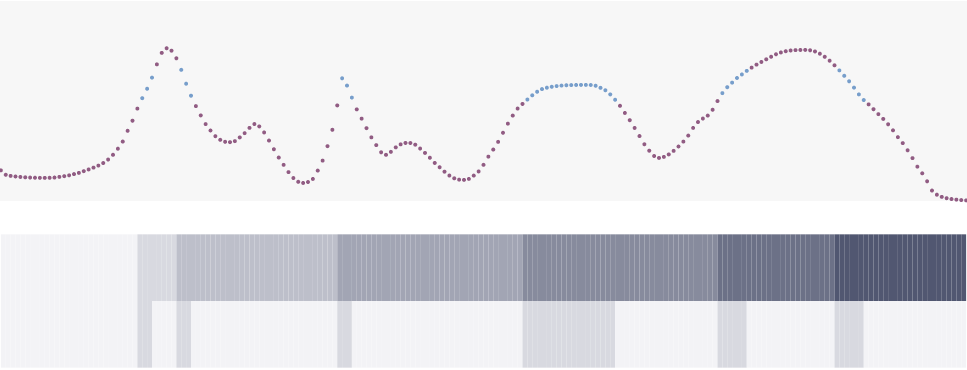
To see this working on a real-world task, I’ve trained a gated RNN on the language modeling problem from this practical. Everything is the same as before, but the \(x_t\) are now words, which are one-hot vectors in \(\mathbb{R}^{V}\), and the features \(h_t\) are passed into linear classifiers to predict the word \(x_{t + 1}\).
Rows of the \(h_t\) that are constant over regions are examples of memory in action.
-
For that matter, the videos themselves are sequences of image frames. ↩
-
Independent and identically distributed, sometimes called “the big lie of machine learning.” ↩
-
It turns out that the state-of-the-art are just clever combinations of these core components, anyways. ↩
-
Notice that this definition doesn’t have any parameters, the notation \(\theta\) is actually superfluous here. ↩
-
In theory, we could use a linear layer to get integer counts. But this would violate the principle of creating generic architectures, which discover features with minimal hand-crafted input. ↩
-
Some of the most compelling graphics are the least intricate! ↩
-
These are cool-kids shorthand for the otherwise dissonant phrases “Long Term Short Term Memory” and “Gated Recurrent Units.” Don’t worry about the names, we’ll explain the math in a second, at least for GRUs. ↩
-
Believe me, if I could, I would. ↩
Kris at 13:43