Borel-Kolmogorov Paradox
Let points be uniformly distributed on the surface of a sphere in $\mathbb{R}^{3}$. Two natural questions of conditional probability are
- How are points distributed, conditional on their lying on a particular latitude?
- Alternatively, how are points distributed conditional on their lying on a given longitude?
The Borel-Kolmogorov paradox is that these distributions are not the same! In this post, we derive this counterintuitive result and supply an illustrative simulation.
Derivation
Without loss of generality, assume that the sphere is the unit sphere. We convert to spherical coordinates, letting $\varphi$ denote the angle between a point and the $z$-axis and $\theta$ denote the angle that the projection of the point into the $xy$-plane makes with the $x$-axis. Notice that $\varphi$ and $\theta$ represent particular lattitudes and longitudes, respectively. From figure 1, we see that we can parameterize the surface of the unit sphere by
\(\begin{align} r(\varphi, \theta) &= \begin{pmatrix} cos\varphi cos\theta \\\ cos\varphi sin\theta \\\ sin\varphi \end{pmatrix}, \end{align}\) where $\varphi \in \left[-\frac{\pi}{2}, \frac{\pi}{2}\right], \theta \in [0, 2\pi)$.

In order to obtain the conditional distributions of interest, we first determine the joint distribution of $\left(\varphi, \theta\right)$, that is, a function $f_{\Phi, \Theta}\left(\varphi, \theta\right)$ such that $\int_{0}^{2\pi}\int_{-\frac{\pi}{2}}^{\frac{\pi}{2}} f_{\Phi, \Theta}\left(\varphi, \theta\right) d\varphi d\theta = 1$.
To this end, either recall from multivariable calculus that the surface area of the unit sphere can be found as $4\pi = \int \int \left|\frac{\partial r}{\partial \varphi} \times \frac{\partial r}{\partial \theta}\right| d\varphi d \theta$, or consider the following argument. At any point $r\left(\varphi, \theta\right)$ on the surface of the sphere, we can form an infinitesimally small parallelogram with edges $\frac{\partial r\left(\varphi, \theta\right)}{\partial \varphi} d\varphi$ and $\frac{\partial r\left(\varphi, \theta\right)}{\partial \theta} d\theta$ that closely approximates the surface at that point. The area of this parallelogram can be found as by the square root determinant of the Gramian of its edges,
\[\begin{align} \sqrt{ \det G\left(\frac{\partial r\left(\varphi, \theta\right)}{\partial \theta} d\varphi, \frac{\partial r\left(\varphi, \theta\right)}{\partial \theta}d\theta\right)} &= \sqrt{\det \begin{pmatrix} \frac{\partial r}{\partial \varphi} d\varphi \\ \frac{\partial r}{\partial \theta} d\theta \end{pmatrix}^{T} \begin{pmatrix} \frac{\partial r}{\partial \varphi} d\varphi \\ \frac{\partial r}{\partial \theta} d\theta \end{pmatrix}} \\ &= \sqrt{\cos^{2}\varphi} d\varphi d\theta. \end{align}\]Integrating over all such infinitesimal parallelograms yields
\[4\pi = \int_{0}^{2\pi}\int_{-\frac{\pi}{2}}^{\frac{\pi}{2}} cos \varphi d\varphi d\theta,\]so we can conclude that the joint density of $\varphi, \theta$ is
\[f_{\Phi, \Theta}\left(\varphi, \theta\right) = \frac{\cos\varphi}{4\pi}.\]The marginal and conditional densities then follow easily by integration:
\[\begin{align} f_{\Phi}\left(\varphi\right) &= \frac{\cos\varphi}{2} \\ f_{\Theta}\left(\theta\right) &=\frac{1}{2\pi} \\ f_{\Phi \mid \Theta}\left(\varphi \mid \theta\right) &= \frac{\cos\varphi}{2} \\ f_{\Theta \mid \Phi}\left(\theta \mid \varphi\right) &= \frac{1}{2\pi}. \end{align}\]Hence, fixing a lattitude, the points are distributed uniformly around the associated horizontal ring, while fixing a longitude, they are distributed according to $\frac{\cos \varphi}{2}$. In particular, conditional on lying on a given longitude, they are more likely to fall near the equator than the poles. In hindsight, this seems reasonable, since the angle $\varphi$ sweeps out a greater length near the equator than the poles. A number of other explanations have been put forth, highlighting the difficulty of conditioning on a set of measure zero and motivating the development of rigorous conditional probability, see for example Jaynes, Kolmogorov, or Manton.
Illustration
We generate $n$ points uniformly on the surface of the sphere using the function
rsphere and convert to coordinates $\varphi$ and $\theta$ using
sphere.coord. The function rsphere uses the fact that, since the standard
Gaussian density is spherically symmetric, taking the projection of Gaussian
points onto the surface of the sphere yields points uniformly distributed on
it. The function sphere.coord uses the transform
\(\begin{align}
\varphi &= \arcsin\left(z\right) \\\
\theta &= \arctan\left(\frac{y}{x}\right),
\end{align}\)
which follows from the parametrization $r\left(\varphi, \theta\right)$.
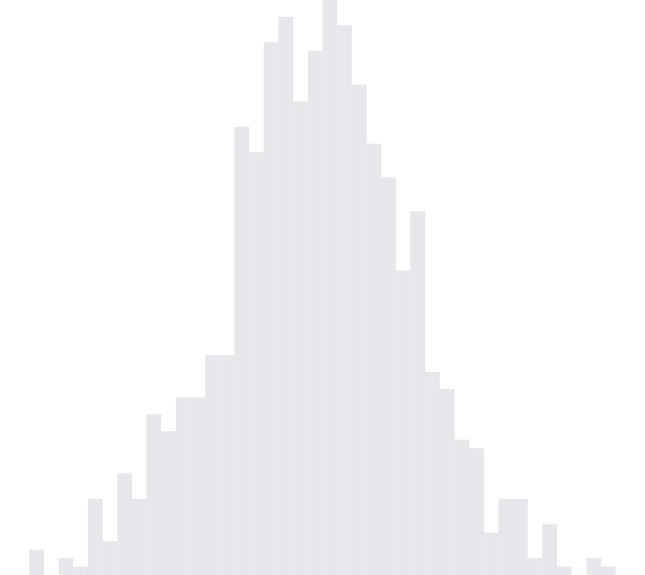
Figure 2 shows the points
on the sphere surface. We can view the joint distribution of points in figure 3 and the associated marginal densities in figure 4. The results confirm the mathematical derivation above.
rsphere <- function(n) {
    X <- matrix(rnorm(n * 3), n, 3)
    X.sphere <- apply(X, MARGIN = 1, FUN = function(x) {
        x/norm(as.matrix(x), "2")
    })
    rownames(X.sphere) <- c("x", "y", "z")
    return(t(X.sphere))
}

X <- rsphere(10000)
library(rgl)
plot3d(X)

You must enable Javascript to view this page properly.
sphere.coord <- function(X) {
    sphere.coord.point <- function(x) {
        phi <- asin(x[3])
        theta <- atan(x[2]/x[1])
        return(c(phi, theta))
    }

    X.coord <- data.frame(t(apply(X, MARGIN = 1, FUN = sphere.coord.point)))
    colnames(X.coord) <- c("phi", "theta")
    return(X.coord)
}

X.tilde <- sphere.coord(X)library(ggplot2)
library(reshape2)
ggplot(X.tilde) + geom_point(aes(x = phi, y = theta))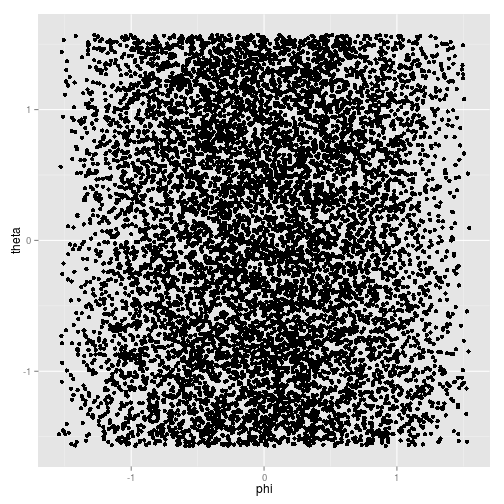
mX <- melt(X.tilde, variable.name = "Coordinate")
ggplot(mX) + geom_histogram(aes(x = value)) + facet_grid(~Coordinate)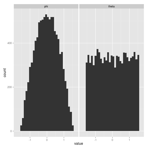
Kris at 00:00