- Even if we can effectively draw curves through data, we might not actually be able to make good predictions on future samples. For example, suppose we fit this complicated curve to a training dataset,
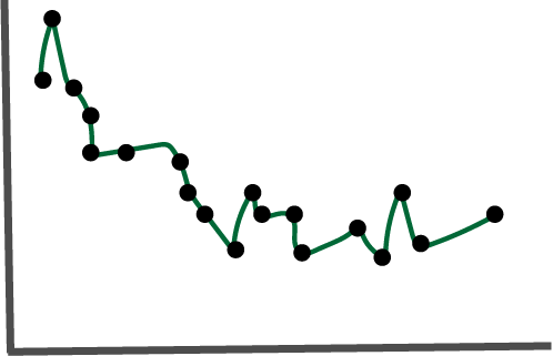
It would have perfect performance on the training data. Now imagine that we collected a few more samples, all from the same population,
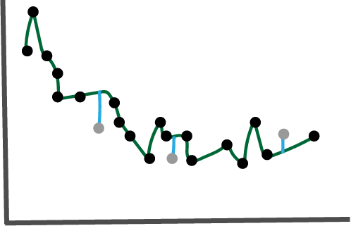
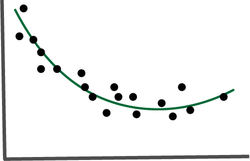
It turns out that the error is higher than a smoother curve that has higher training error,
Notice that the blue test errors are all shorter here than in the previous fit,

- This issue can also occur in classification. For example, the decision boundary here,

is perfect on the training dataset. But it will likely perform worse than the simpler boundary here,

This phenomenon is called overfitting. Complex models might appear to do well on a dataset available for training, only to fail when they are released “in the wild” to be applied to new samples. We need to be very deliberate about choosing models that are complex enough to fit the essential structure in a dataset, but not so complex that they overfit to patterns that will not appear again in future samples.
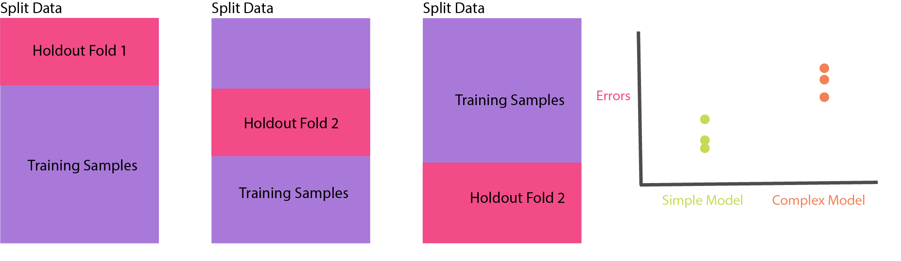
The simplest way to choose a model with the right level of complexity is to use data splitting. Randomly split the data that are available into a train and a test sets. Fit a collection of models, all of different complexities, on the training set. Look at the performances of those models on the test set. Choose the model with the best performance on the test set.

- A more sophisticated approach is to use cross-validation. Instead of using only a single train / test split, we can group the data into \(K\)-different “folds.” For each complexity level , we can train \(K\) models, each time leaving out one of the folds. Performance of these models on the hold-out folds is used for estimating the appropriate complexity level.
- There are a few subtleties related to train / test splits and cross-validation that are worth knowing,
- We want the held-out data to be as representative of new, real-world data as possible. Sometimes, randomly split data will not be representative. For example, maybe the data are collected over time. A more “honest” split would split data into past vs. future samples starting at a few different timepoints, training on past and evaluating on future. The sample issue occurs if we plan on applying a model to a new geographic context or market segment, for example.
- Cross-validation can be impractical on larger datasets. For this reason, we often see only a single train / test split for evaluation of algorithms in large data settings.
- We incur a bias when splitting the data. The fact that we split the data means that we aren’t using all the available data, which leads to slightly lower performance. If it hurts more complex models more than simpler ones, than it can even lead to slightly incorrect selection. After having chosen a given model complexity, it’s worth retraining that model on the full available dataset.
- Let’s implement both simple train / test and cross-validation using
sklearn. First, let’s just use a train / test split, without cross-validating. We’ll consider the penguins dataset from the earlier lecture.
from sklearn.model_selection import train_test_split
import pandas as pd
import numpy as np

# prepare data
penguins = pd.read_csv("https://uwmadison.box.com/shared/static/mnrdkzsb5tbhz2kpqahq1r2u3cpy1gg0.csv")
penguins = penguins.dropna()
X, y = penguins[["bill_length_mm", "bill_depth_mm"]], penguins["species"]
(
  X_train, X_test,
  y_train, y_test,
  indices_train, indices_test
) =  train_test_split(X, y, np.arange(len(X)), test_size=0.25)
Let’s double check that the sizes of the train and test sets make sense.
len(indices_train)249len(indices_test)84Now, we’ll train the model on just the training set.
from sklearn.ensemble import GradientBoostingClassifier

model = GradientBoostingClassifier()
model.fit(X_train, y_train)GradientBoostingClassifier()penguins["y_hat"] = model.predict(X)
# keep track of which rows are train vs. test
penguins["split"] = "train"
penguins = penguins.reset_index()
penguins.loc[list(indices_test), "split"] = "test"Finally, we’ll visualize to see the number of errors on either split. The first row are the test samples, the second row are the train samples. Notice that even though prediction on the training set is perfect, there are a few errors on the test set.
ggplot(py$penguins) +
  geom_point(aes(bill_length_mm, bill_depth_mm, col = species)) +
  scale_color_manual(values = c("#3DD9BC", "#6DA671", "#F285D5")) +
  labs(x = "Bill Length", y = "Bill Depth") +
  facet_grid(split ~ y_hat)
- Next, let’s look at cross validation. There is a handy wrapper function called
cross_val_scoreinsklearnthat handles all the splitting and looping for us. We just have to give it a model type and it will evaluate it on a few splits of the data. Thescoresvector below gives the error rate on \(K = 5\) holdout folds.
from sklearn.model_selection import cross_val_score
model_class = GradientBoostingClassifier()
scores = cross_val_score(model_class, X, y, cv=5)
scores
array([1. , 0.98507463, 0.94029851, 0.90909091, 0.96969697])- Related to overfitting, there is an important phenomenon called the bias-variance tradeoff. To understand this trade-off, imagine being able to sample hundreds of datasets similar to the one that is available. On each of these datasets, we can train a new model (at a given complexity level). Then, we can define,
- Bias: Average the predictions from models trained across each of the imaginary datasets. How far off are they from the truth, on average?
- Variance: How similar are predictions from across the different runs?
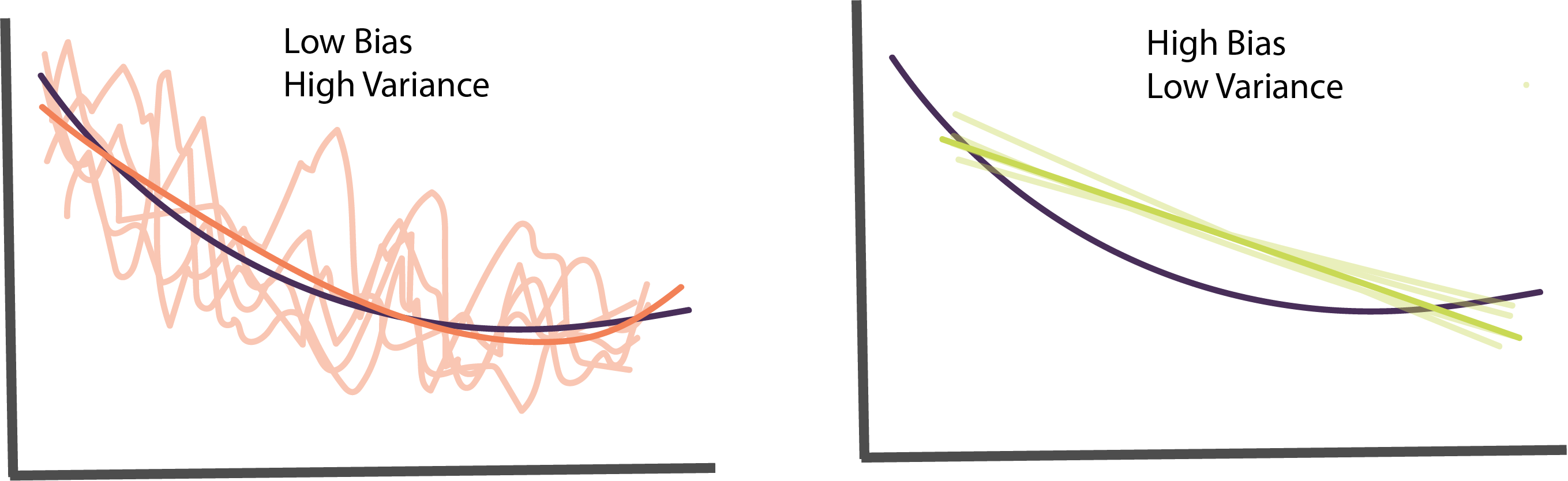
Ideally, we would have low values for both bias and variance, since they both contribute to performance on the test set. In practice, though, there is a trade-off. Often, the high-powered models that tend to be closest to the truth on average might be far off on any individual run (high variance). Conversely, overly simple models that are very stable from run to run might be consistently incorrect in certain regions (bias).
Models with high variance but low bias tend to be overfit, and models with low variance but high bias tend to be underfit. Models that have good test or cross-validation errors have found a good compromise between bias and variance.
In practice, a useful strategy is to,
- Try overfitting the data. This ensures that the features and / or model class are sufficiently rich. This provides a kind of upper bound on the possible performance with the current setup.
- Try regularizing the overfit model so that it also performs well on holdout data.