A few simple improvements to the quality of a dataset can make a bigger impact in downstream modeling performance than even the most extensive search across the fanciest models. For this reason, in real-world modeling (not to mention machine learning competitions), significant time is dedicated to data exploration and preprocessing1. In these notes, we’ll review some of the most common transformations we should consider for a dataset before simply throwing it into a model.
First, a caveat: Never overwrite the raw data! Instead, write a workflow that transforms the raw data into a preprocessed form. This makes it possible to try a few different transformations and see how the resulting performances compare. Also, we want to have some confidence that the overall analysis is reproducible, and if we make irreversible changes to the raw data, then that becomes impossible.
Preprocessing
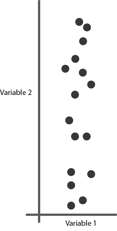
- Outliers: A single point very far away from the rest can result in poor fits. For example, when fitting a linear regression, the whole line can be thrown off by one point,
](figures/outlier-influence.png)
Figure 1: Figure from this site
There are many approaches to detecting outliers. However, a simple rule of thumb is to compute the interquartile range for each feature (the difference between the 75% and 25% percentiles). Look for points that are more than 1.5 or 2 times this range away from the median. They are potential outliers.
- Differences in scales: Sparse regression is sensitive to the units used to train them (so is deep learning). For example, this means that changing the units of a certain input from meters to millimeters will have a major influence on the fitted model. To address this issue, it is common to try rescaling each variable. For example, subtracting the mean and dividing by the standard deviation will ensure all the variables have approximately the same range. It’s also possible to convert any variable \(x_{d}\) to the range \(\left[0, 1\right]\) by using the transformation \(\frac{x - x_{\text{min}}}{x_{\text{max}} - x_{\text{min}}}\).
- Missing values: For some types of data, features have to be dropped for some samples. The sensor might have a temporary breakdown, or a respondent might have skipped a question, for example. Unfortunately, most methods do not have natural ways for handling missingness. To address this, it’s possible to impute a plausible value for all the missing values. A standard approach to imputation is to replace the missing values in a column using the median of all observed values in that column. This is called median imputation.

More sophisticated approaches are able to learn the relationships across columns, and use these correlations to learn better imputations. This is called multiple imputation.
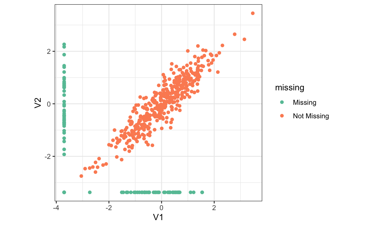
Figure 2: An example where correlation between two variables might be used to impute their missing values (when exactly one is present).
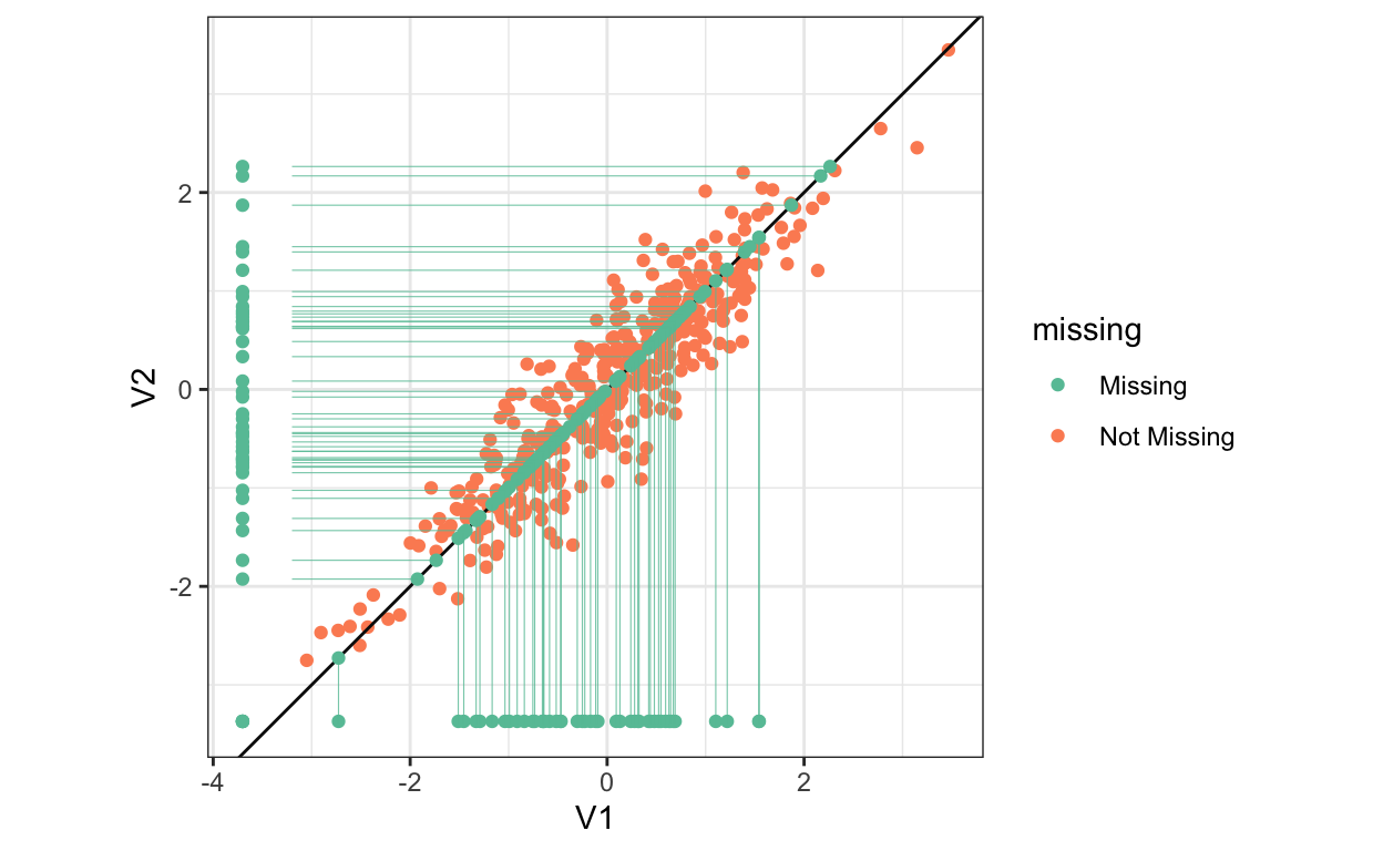
Figure 3: Imputations using multiple imputation.
Be especially careful with numerical values that have been used as a proxy for missingness (e.g., sometimes -99 is used as a placeholder). These should not be treated as actual numerical data, they are in fact missing!
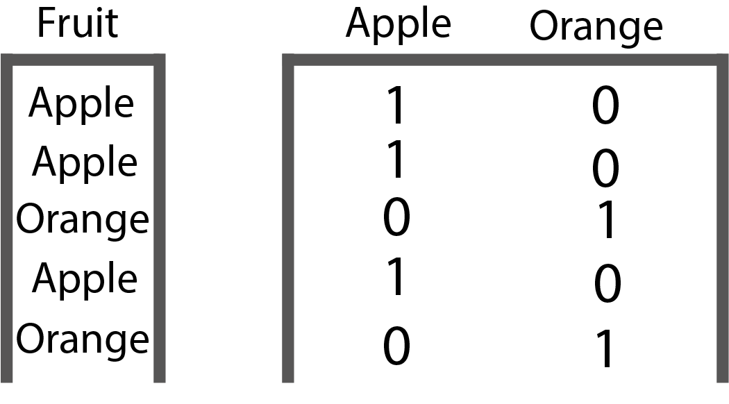
- Categorical inputs: From the last set of notes, only tree-based methods can directly use categorical variables as inputs. For other methods, the categorical variables needed to be coded. For example, variables with two levels can be converted to 0’s and 1’s, and variables with \(K\) levels can be one-hot coded,
Sometimes a variable has many levels. For example, a variable might say which city a user was from. In some cases, a few categories are very common, with the rest appearing only a few times. For the first situation, one solution is to replace the level of the category with the average value of the response within that category – this is called response coding. For the second, it’s possible to lump all the rare categories into an “other” column.
- To detect the types of issues discussed here, a good practice is to compute (i) summary statistics and (ii) a histogram / barplot for every feature in the dataset. Even if there are a few hundred features, it’s possible to skim the associated summaries relatively quickly (just a few seconds for each).
Featurization
- Often, useful predictors can be derived from, but are not explicitly present in, the raw data. For example, linear regression would struggle with either of the cases below,

but if we add new columns to the original data \(x\),
\[\begin{align*} \begin{pmatrix} x & x^2 \end{pmatrix} \end{align*}\]
or
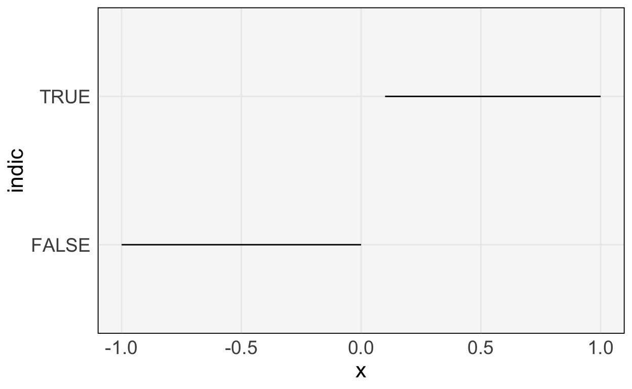
\[\begin{align*} \begin{pmatrix} x & \mathbf{1}\left\{x > 0\right\} \end{pmatrix} \end{align*}\]
we will be able to fit the response well. The reason is that, even though \(y\) is not linear in \(x\), it is linear in the derived features \(x^2\) and \(\mathbf{1}\left\{x > 0\right\}\), respectively.
- This idea applies to all sorts of data, not just numerical columns,
- Longitudinal measurements: Imagine we want to classify a patient’s recovery probability based on a series of lab test results. We don’t have to use the raw measurements, we can use the trend, the range, or the “spikiness,” for example.
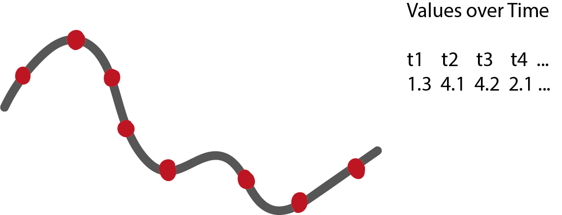
Figure 4: The raw measurements associated with a series. Imagine that we need to classify these series into groups with different shapes.
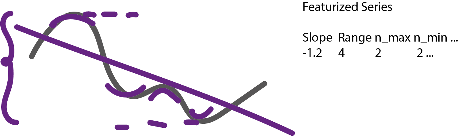
Figure 5: An example featurization of a longitudinal series.
- Text: We can convert a document into the counts for different words.
- Images: For some tasks, the average color can be predictive (imagine classifying scenes as either forest or beach, which do you think will have more green on average?).

The difficulty of deriving useful features in image data was one of the original motivations for deep learning. By automatically learning relevant features, deep learning replaced a whole suite of more complicated image feature extractors (e.g., HOG and SIFT).