Interactive Visualization of Metric Distortion in Nonlinear Data Embeddings using the distortions Package

Kris Sankaran

University of Wisconsin-Madison

measurement-and-microbes.org

SDSS 2026

go.wisc.edu/9g3mce

2026-04-30

Dimensionality Reduction

Modern omics data have many features, and dimensionality reduction methods help create overview visualizations.

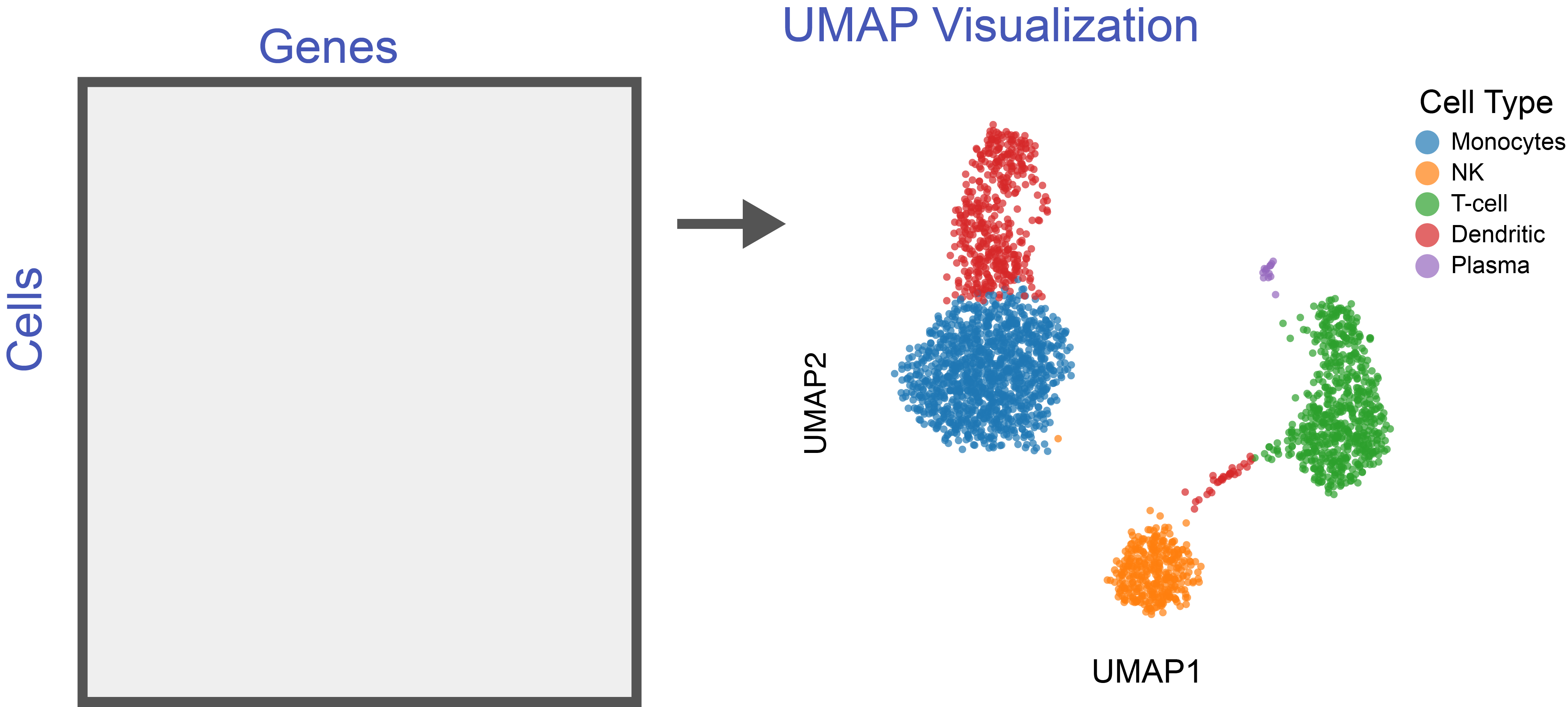
They are also used in cell atlas construction and trajectory inference.

\(\def\Dir{\text{Dir}}\) \(\def\Mult{\text{Mult}}\) \(\def\*#1{\mathbf{#1}}\) \(\def\m#1{\boldsymbol{#1}}\) \(\def\Unif{\text{Unif}}\) \(\def\win{\tilde{w}_{\text{in}}}\) \(\def\reals{\mathbb{R}}\) \(\newcommand{\wout}{\tilde w_{\text{out}}}\)

Distortions in \(t\)-SNE and UMAP

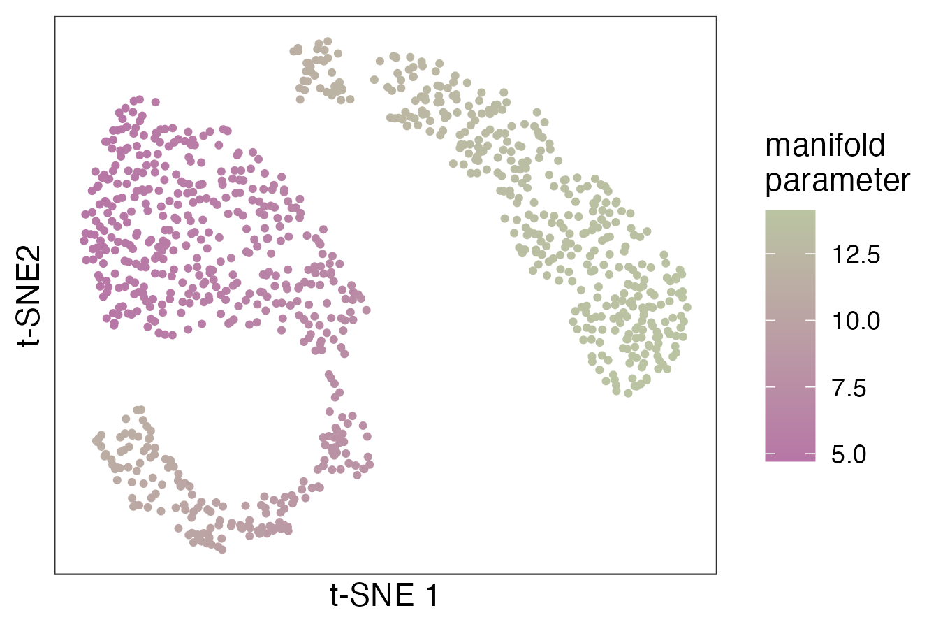
Both \(t\)-SNE and UMAP introduce distortions. For example, they may not preserve density within different regions of the plot.

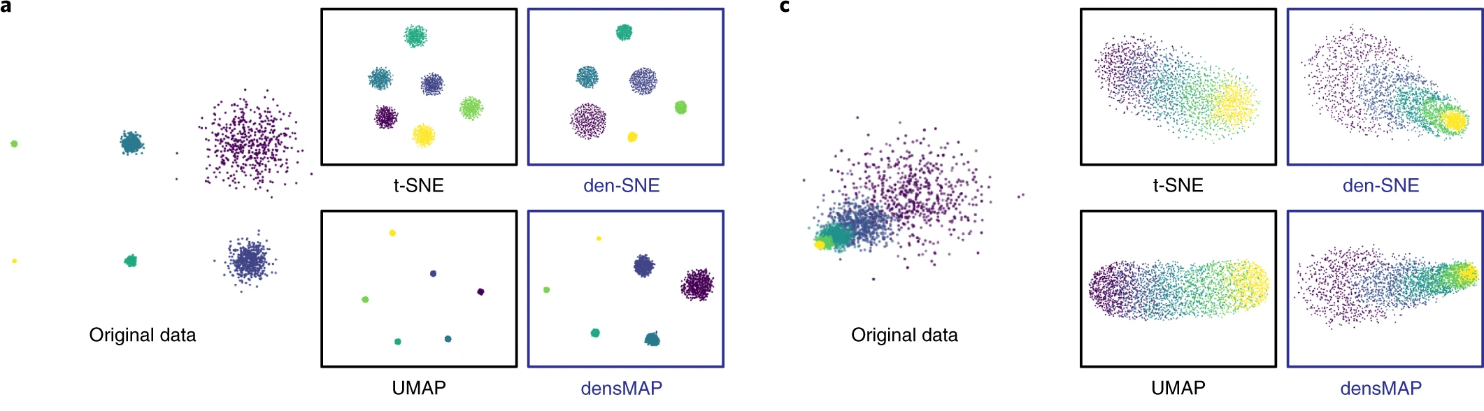
Example from (Narayan, Berger, and Cho 2021).

Distortions in \(t\)-SNE and UMAP

They can also fail to preserve the topology of the underlying data…

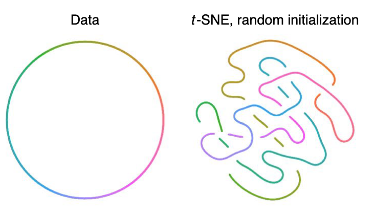
Example from (Kobak and Linderman 2021).

Consequences

These distortions are not mere technical curiosities – they significantly impact scientific interpretation (Liu, Ma, and Zhong 2025; Kobak and Linderman 2021). For example, they create misleading differences between cell types that are actually similar.

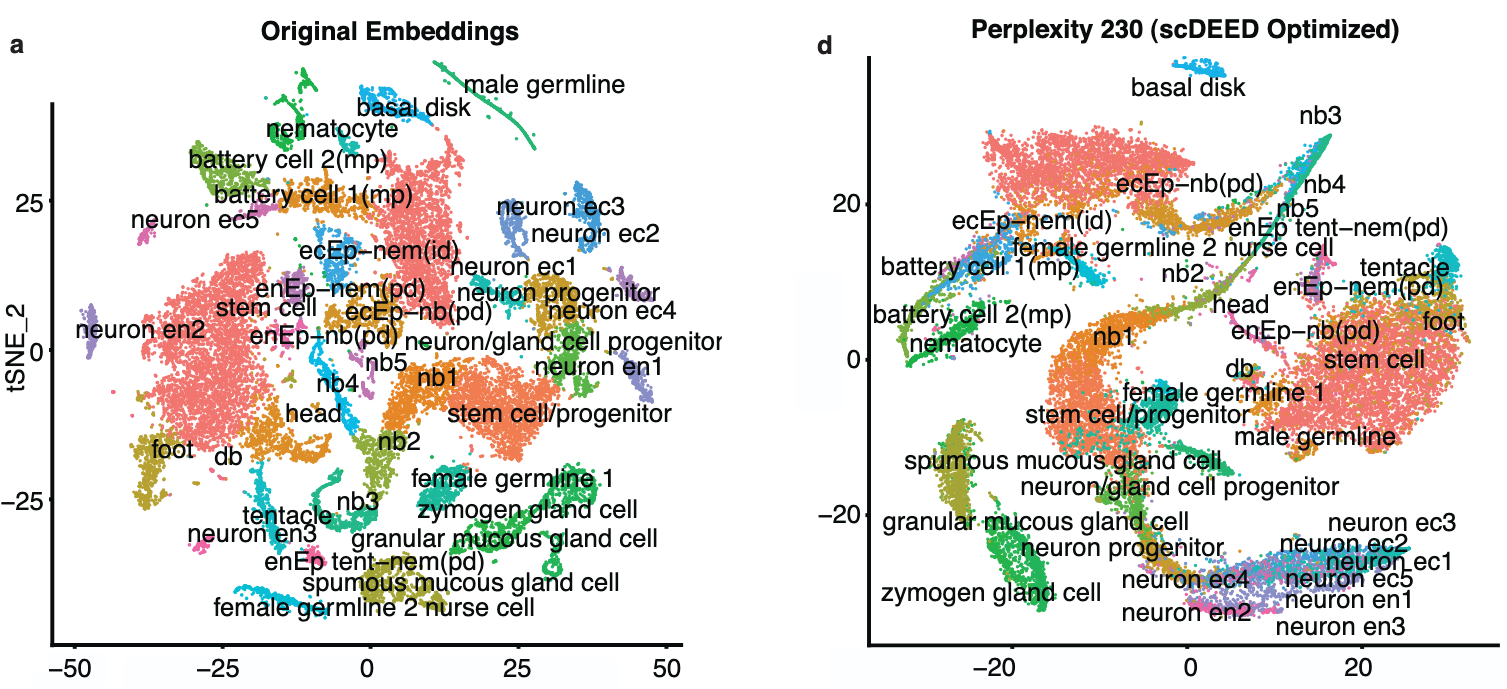Example from (Xia, Lee, and Li 2024).

Approach

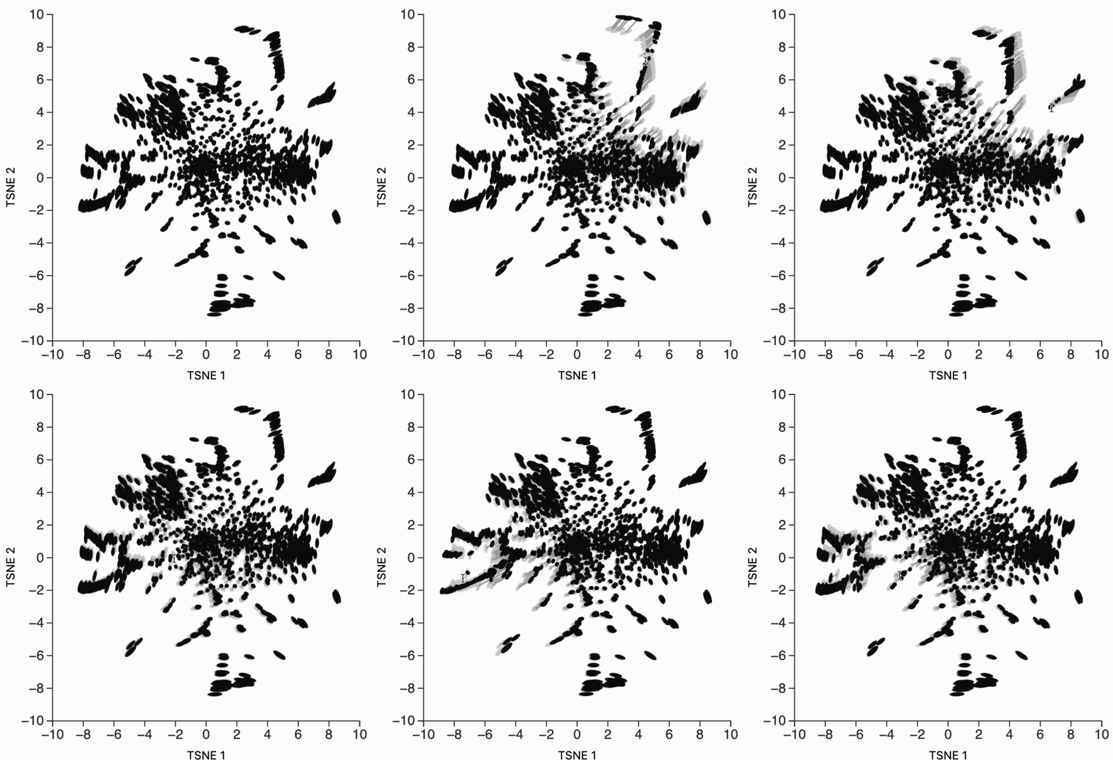
Rather than abandoning nonlinear dimensionality reduction, we augment the embeddings to characterize distortion.

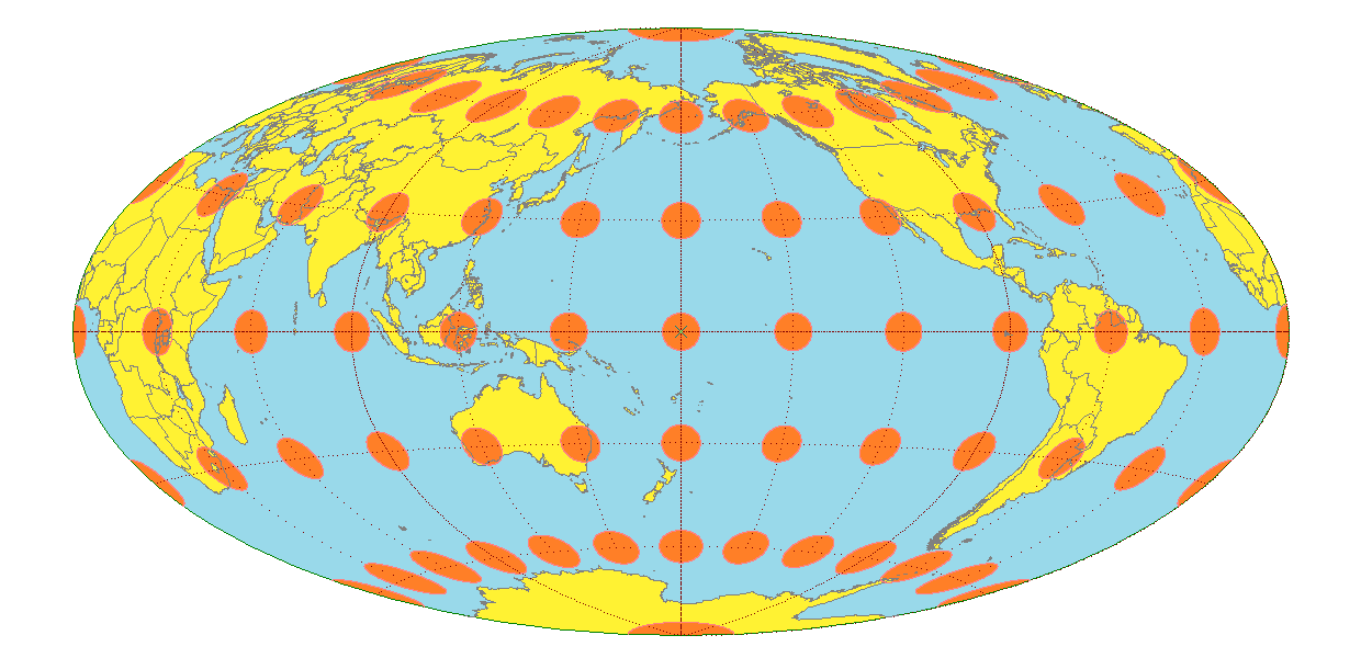
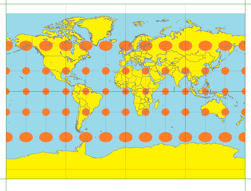
This is a high-dimensional version of Tissot’s indicatrix from cartography (Laskowski 1989).

RMetric Motivation

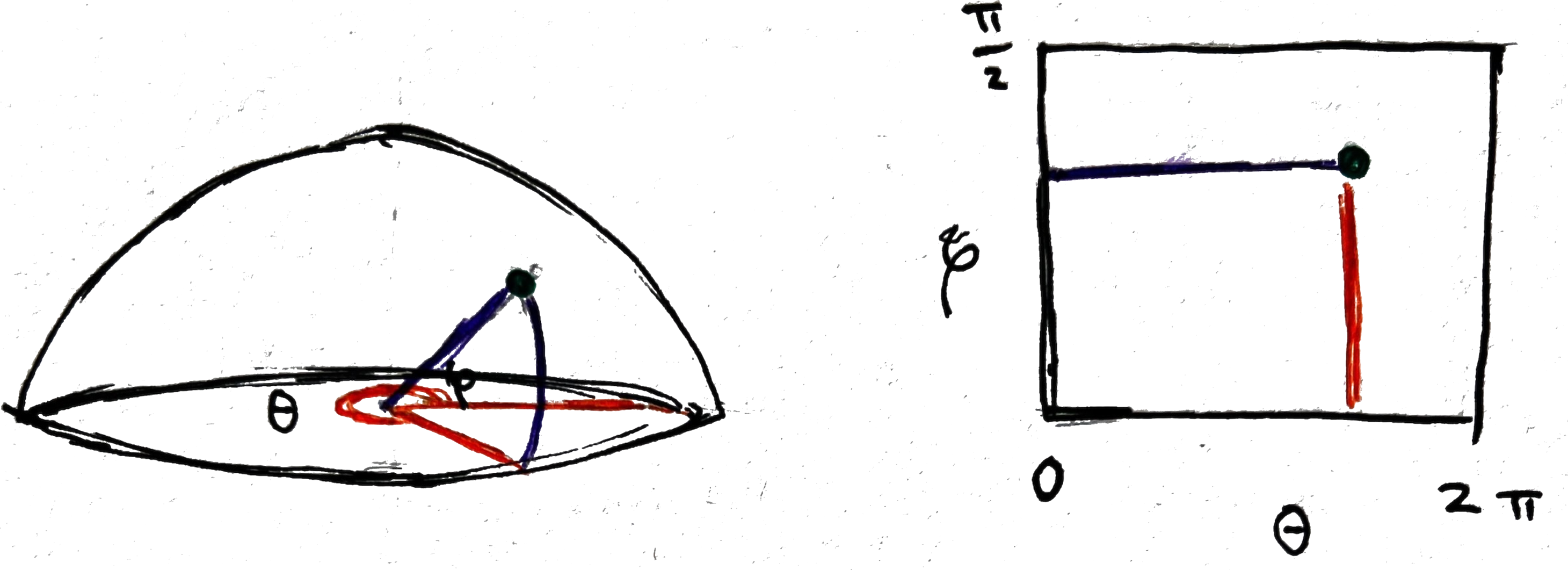
The RMetric algorithm (Perrault-Joncas and Meila 2006; McQueen et al. 2016) quantifies distortion geometrically. To motivate the algorithm, consider the distortion induced by mapping the sphere into latitude/longitude coordinates.

Half-Sphere Parameterization

Parameterize points on \(\mathcal{M}\) using spherical coordinates:

\[\begin{align*} \mathbf{x}\left(p\right) = \left(\cos\varphi\cos\theta, \cos\varphi \sin\theta, \sin\varphi\right) \end{align*}\]

The associated (latitude, longitude) embedding is

\[\begin{align*} \mathbf{z}\left(p\right) = \left(\theta\left(p\right), \varphi\left(p\right)\right). \end{align*}\]

Dual Pushforward Metric

The gradients \(\nabla z^i\) of the embedding dimensions reflect distortion.

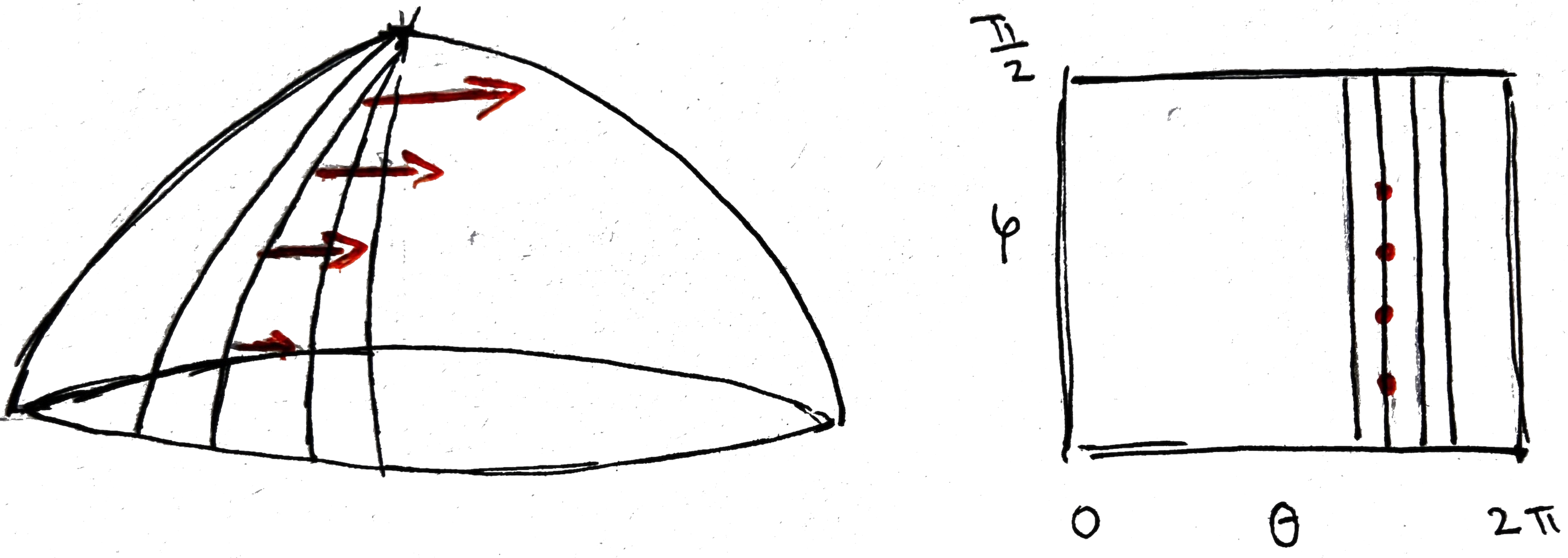
Since the level sets of \(z^\theta\) become more compressed near the poles, the gradients \(\nabla z^\theta\) become larger there.

Dual Pushforward Metric

This gradient information can be stored in the matrix \(H\) with elements,

\[\begin{align*} h^{ij} = \langle \nabla z^i, \nabla z^j \rangle_{g_{0}} \end{align*}\] where \(g_{0}\) is the metric on \(\mathcal{M}\) inherited from the ambient space.

In our example,

\[\begin{align*} H = \begin{pmatrix} 1/\cos^2\varphi & 0 \\ 0 & 1 \end{pmatrix} \end{align*}\]

Product Rule for Laplacians

For any \(f\) and \(g\), the Laplacian \(\Delta\) satisfies, \[\begin{align*} \Delta(fg) = f\,\Delta g + g\,\Delta f + 2\langle \nabla f, \nabla g \rangle_{g_{0}} \end{align*}\]

Setting \(f = z^i\), \(g = z^j\) and rearranging, \[\begin{align*} h^{ij} = \langle \nabla z^i, \nabla z^j \rangle_{g_0} = \frac{1}{2}\left[\Delta(z^i z^j) - z^i\Delta z^j - z^j\Delta z^i\right] \end{align*}\]

Since there are methods for estimating \(\Delta\) from data (Hein, Audibert, and Luxburg 2005; Coifman and Lafon 2006), we also have a practical method for approximating local distortions \(H\).

Implementation

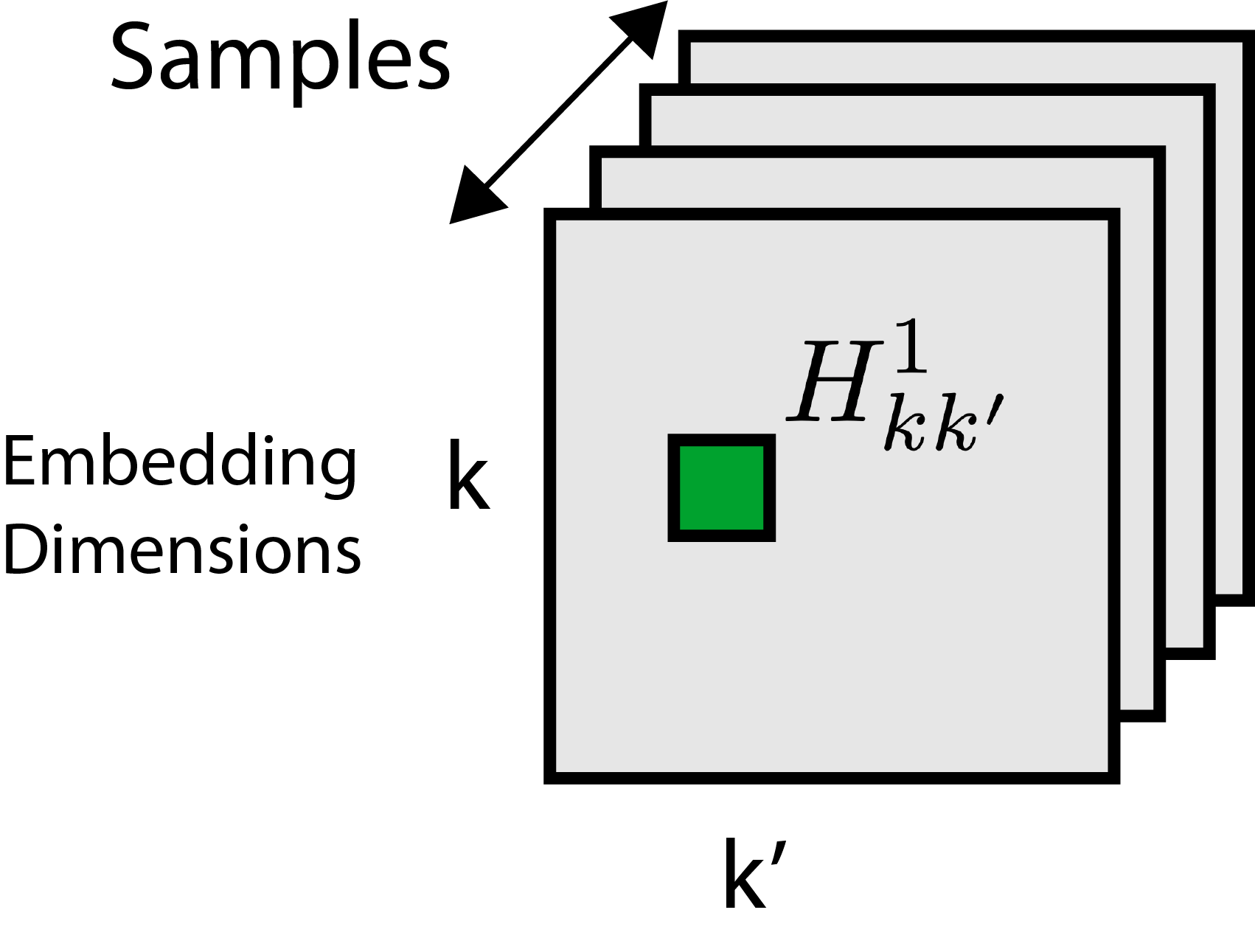
Let \(z_{k} \in \mathbb{R}^{N}\) be the \(k^{th}\) embedding dimension. Let \(L\) be the doubly-normalized graph Laplacian (Coifman and Lafon 2006). Compute

\[\begin{align*} H_{kk'}^{(\cdot)} := \frac{1}{2}\left[L\left(z_{k} \circ z_{k'}\right) - z_{k} \circ \left(L z_{k'}\right) - z_{k'} \circ \left(L z_{k}\right) \right] \in \mathbb{R}^{N} \end{align*}\]

The embedding distortion for sample \(n\) is given by \(H^{(n)} \in \mathbb{R}^{K \times K}\)

Example

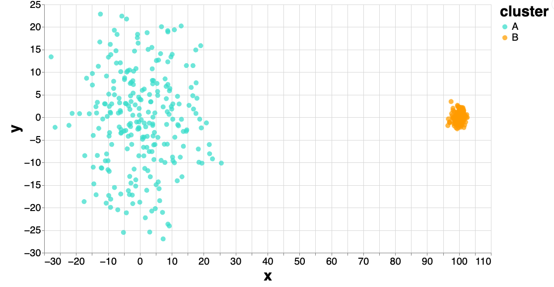
These two clusters are generated as:

\[\begin{align*} x_{i} \sim \frac{1}{2}\mathcal{N}\left(0, 10\right) + \frac{1}{2}\mathcal{N}\left(100, 1\right) \end{align*}\]

Example

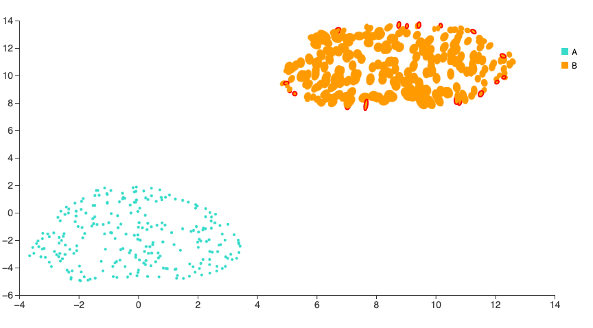
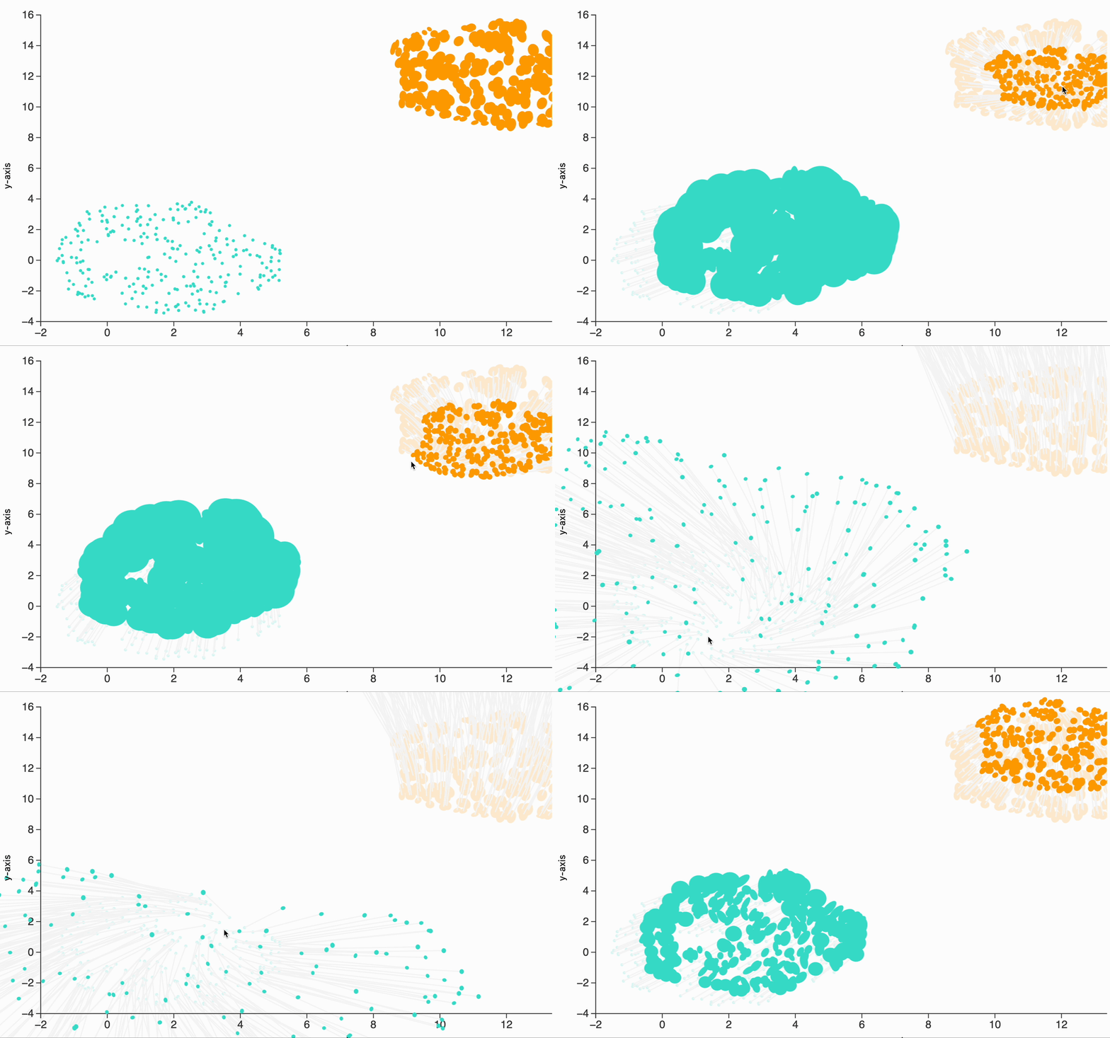
The UMAP embeddings lose information about the cluster density, but the difference is captured in the local metrics.

Local Isometrization

Since the metrics are known locally, the distortion can be inverted within a neighborhood of the cursor. For example, here we interactively adapt the embeddings in the Gaussian mixtures example.

Fragmented Neighborhoods

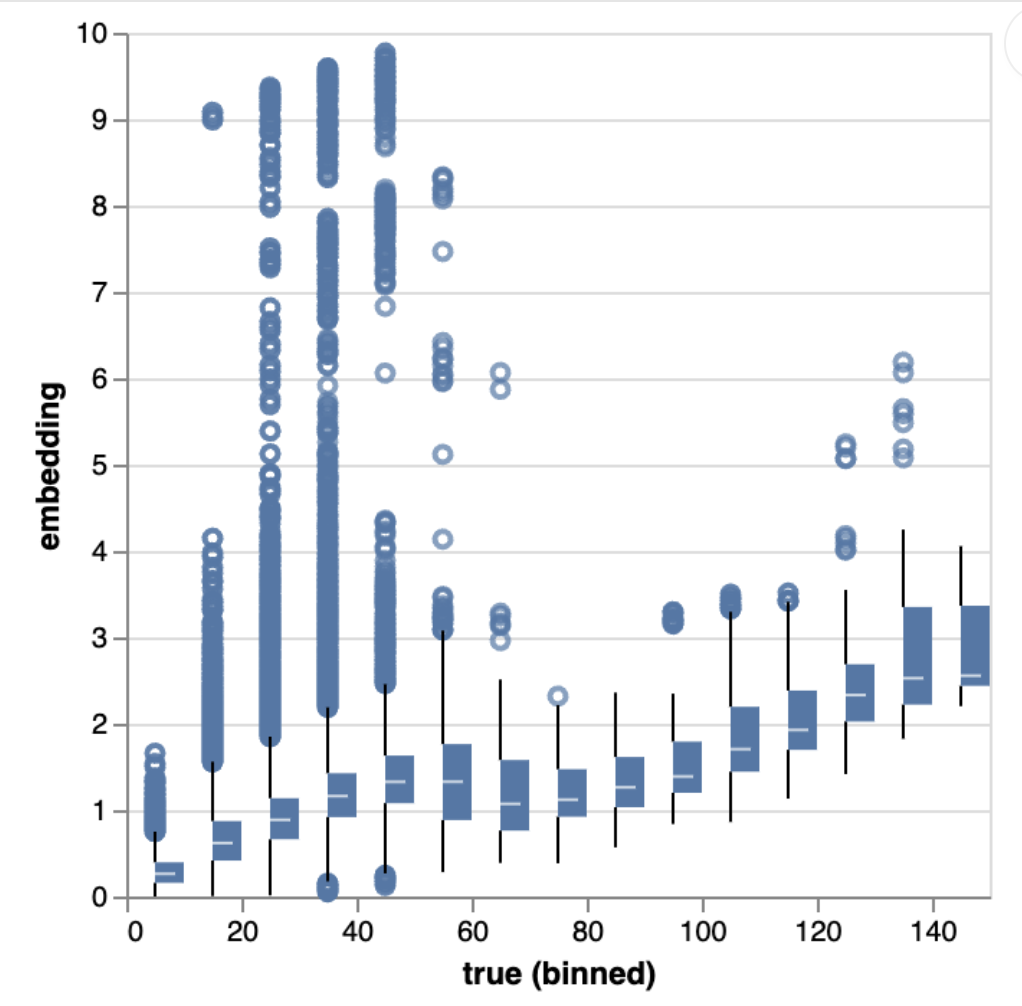
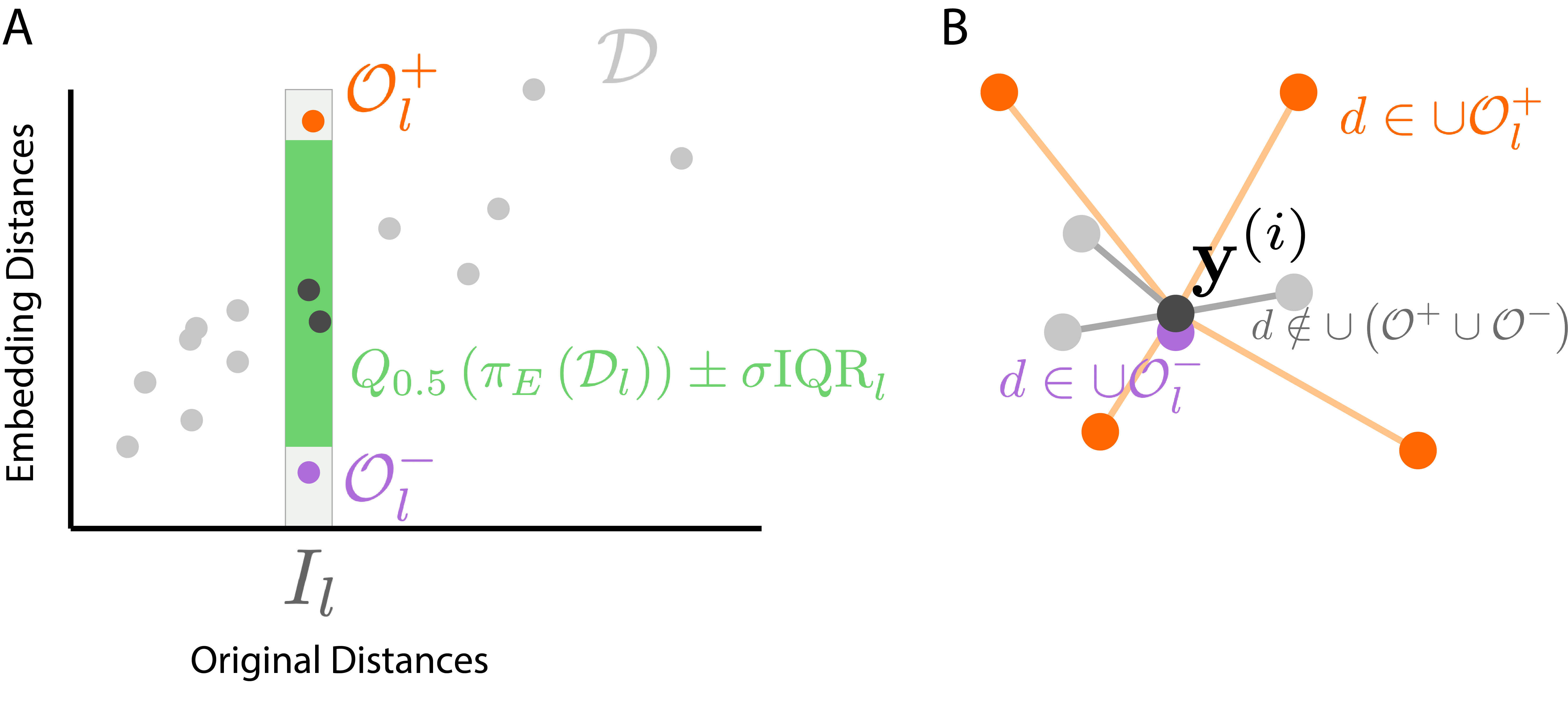
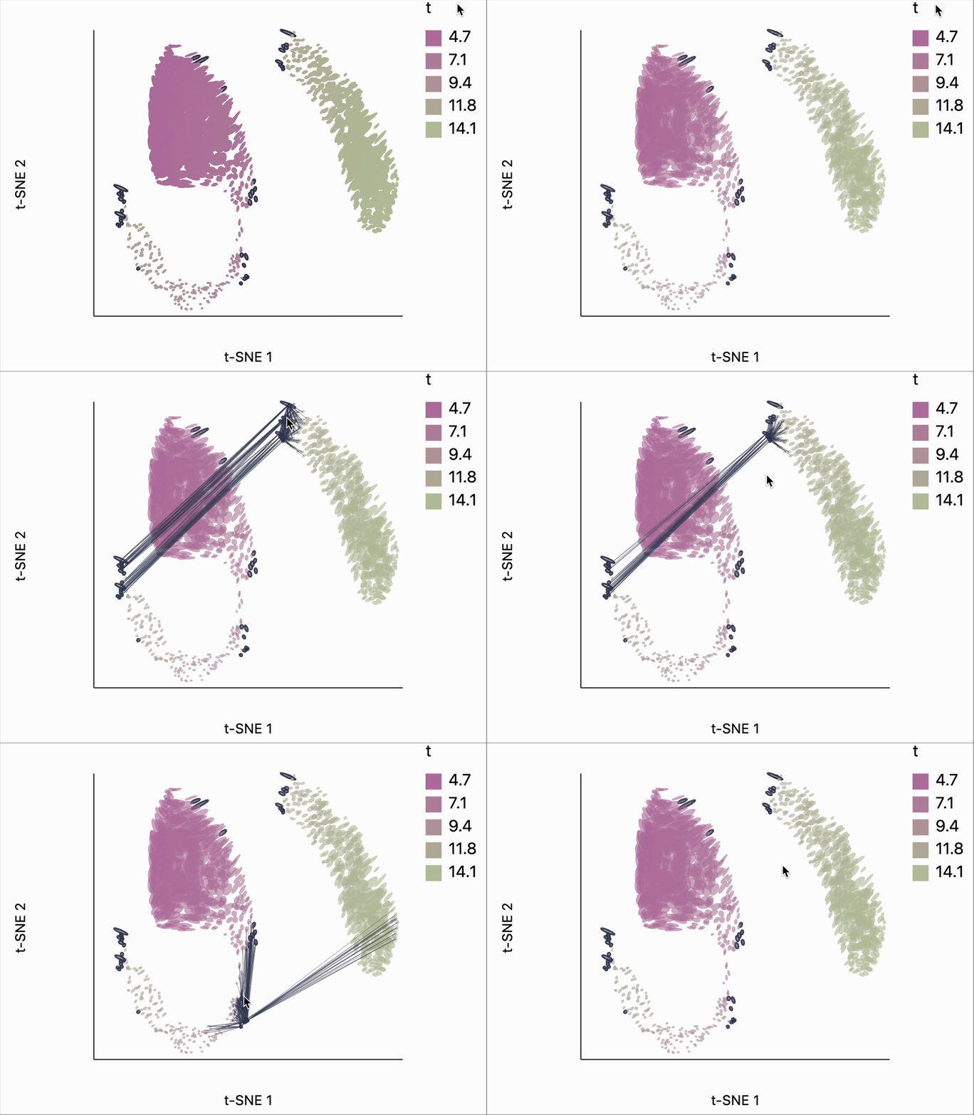
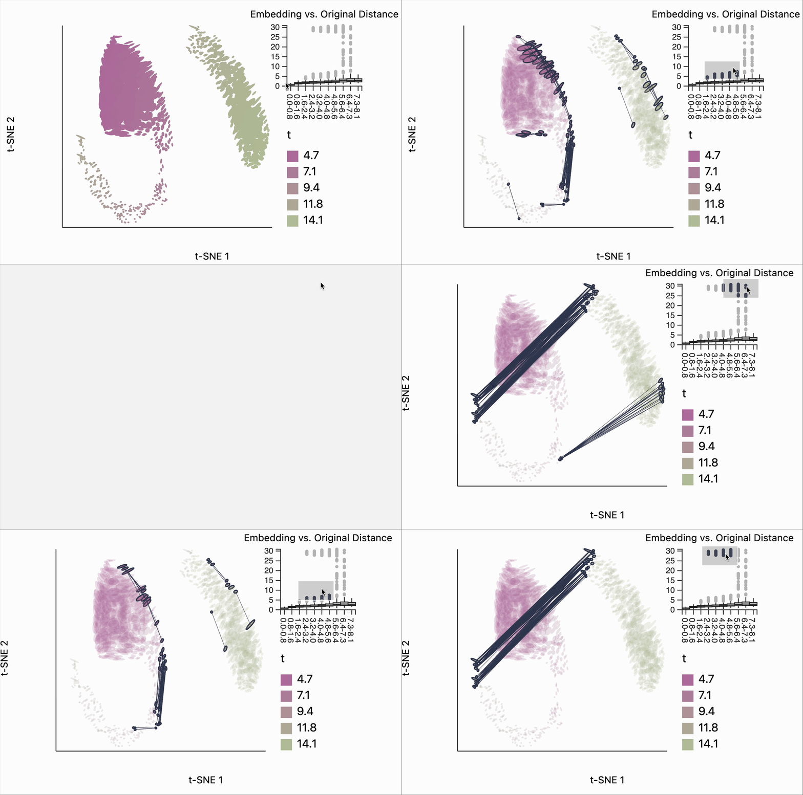
Besides RMetric, we also visualize distortions using the scatterplot of true vs. embedding neighborhood distances.

Fragmented Neighborhoods

To detect poorly preserved neighborhoods, we fit a running median to true vs. embedding distances, flag outliers above \(3\times \text{IQR}\), and mark points with many outlier links as “broken.”

Examples

This is the classic Swiss Roll data, but with higher density near the endpoints.

Variable Density Swiss Roll

\(t\)-SNE (perplexity = 100) breaks the roll in the low-density region and artificially spreads the high density area.

Fragmented Neighborhoods

Poorly Preserved Distances

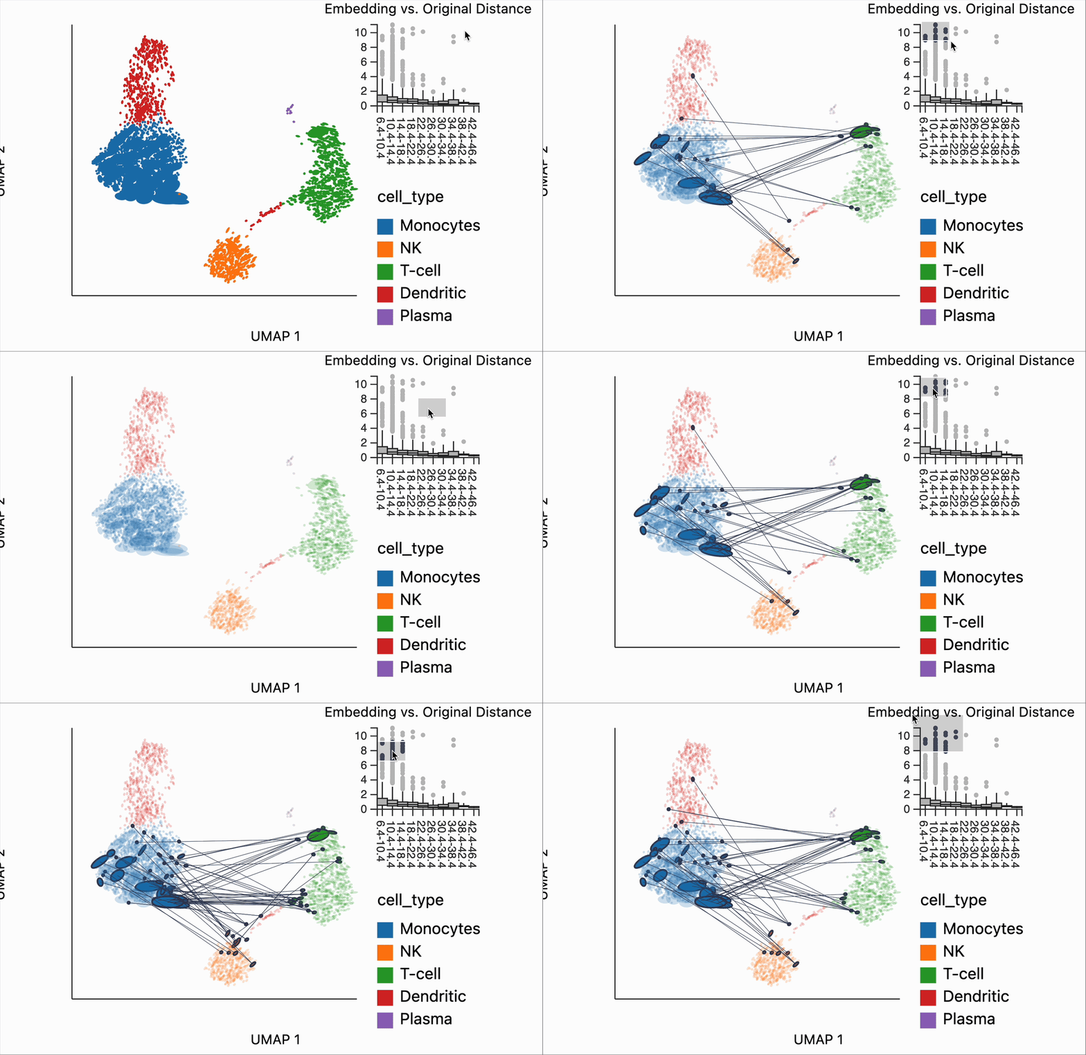
PBMC Dataset

This single-cell gene expression data set was used in the data visualization tutorial from the scanpy package (Wolf, Angerer, and Theis 2018). Each point is the UMAP embedding of a cell’s high-dimensional gene expression data.

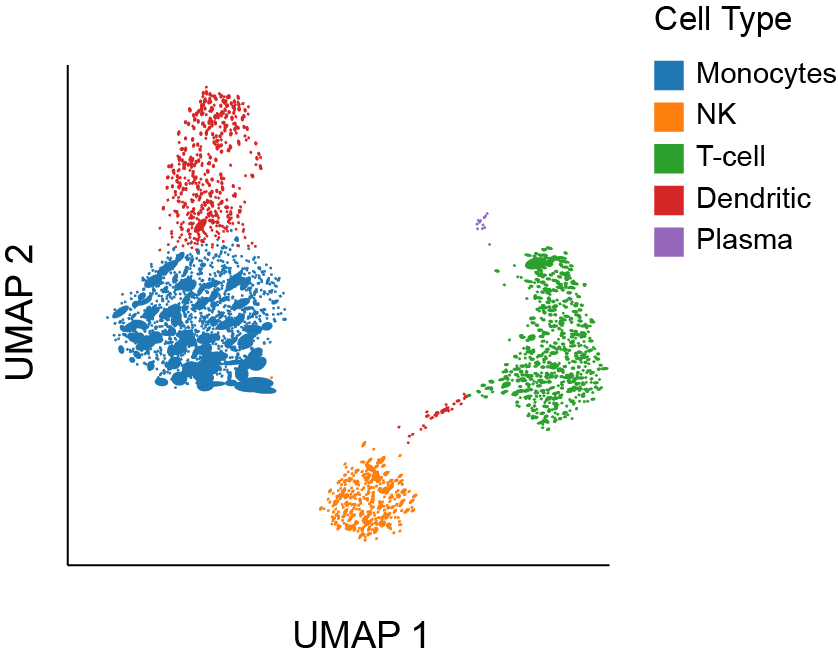
PBMC Dataset

• Distance scales vary both across and within clusters.
• Two T-cell sets appear farther from Monocytes than they actually are.

DensMap vs. UMAP

Both variation in ellipses and fragmented neighborhood statistics can be used to compare competing algorithms, similarly to (Xia, Lee, and Li 2024; Venna and Kaski 2006).

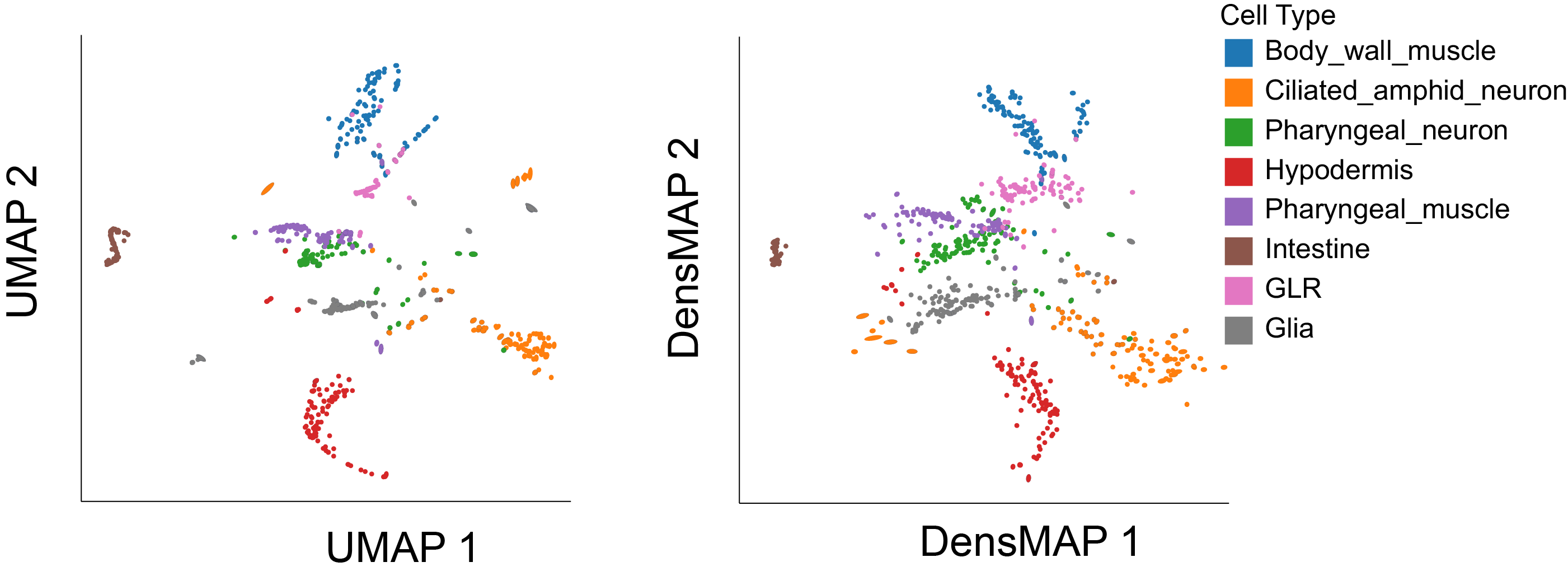
This example uses data from a C. elegans cell differentiation study (Packer et al. 2019).

DensMap vs. UMAP

Both variation in ellipses and fragmented neighborhood statistics can be used to compare competing algorithms, similarly to (Xia, Lee, and Li 2024; Venna and Kaski 2006).

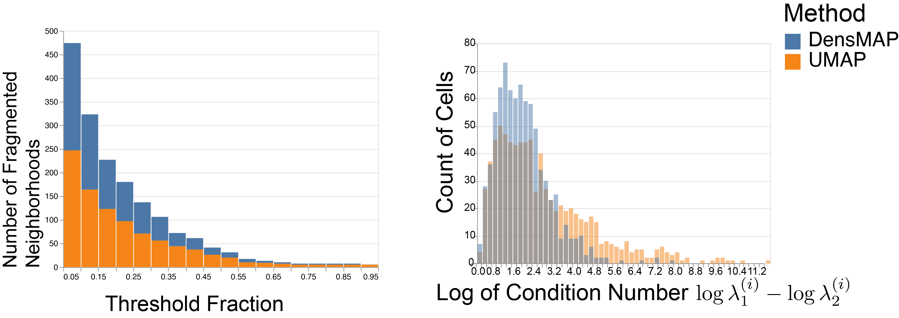
This example uses data from a C. elegans cell differentiation study (Packer et al. 2019).

Summary

Interactivity can reveal distortion information based on the analyst’s priorities.

Paper: https://go.wisc.edu/ptz5j5

Package: https://pypi.org/project/distortions

Sankaran, K., Zhang, S., Chenab, & Meilă, M. (2026). Interactive visualization of metric distortion in nonlinear data embeddings using the distortions package. Briefings in Bioinformatics, 27(2). doi:10.1093/bib/bbag136

Acknowledgments

• Contact: ksankaran@wisc.edu
• Lab Members: Margaret Thairu, Yuliang Peng, Langtian Ma, Cameron Jones, Jiaxin Ye, Megan Kuo, Helena Huang
• Funding: NIGMS R01GM152744, NIAID R01AI184095, Gates INV-072185, NIH R01HG014687

Appendix

Focus-plus-Context

The focus-plus-context principle (Heer and Card 2004) states that readers should be able to zoom into patterns of interest without losing relevant context.

Focus-plus-Context: Barplots

Stacked barplots visualize sample-to-sample variation in microbiome community structure. They struggle to show finer taxonomic resolutions.

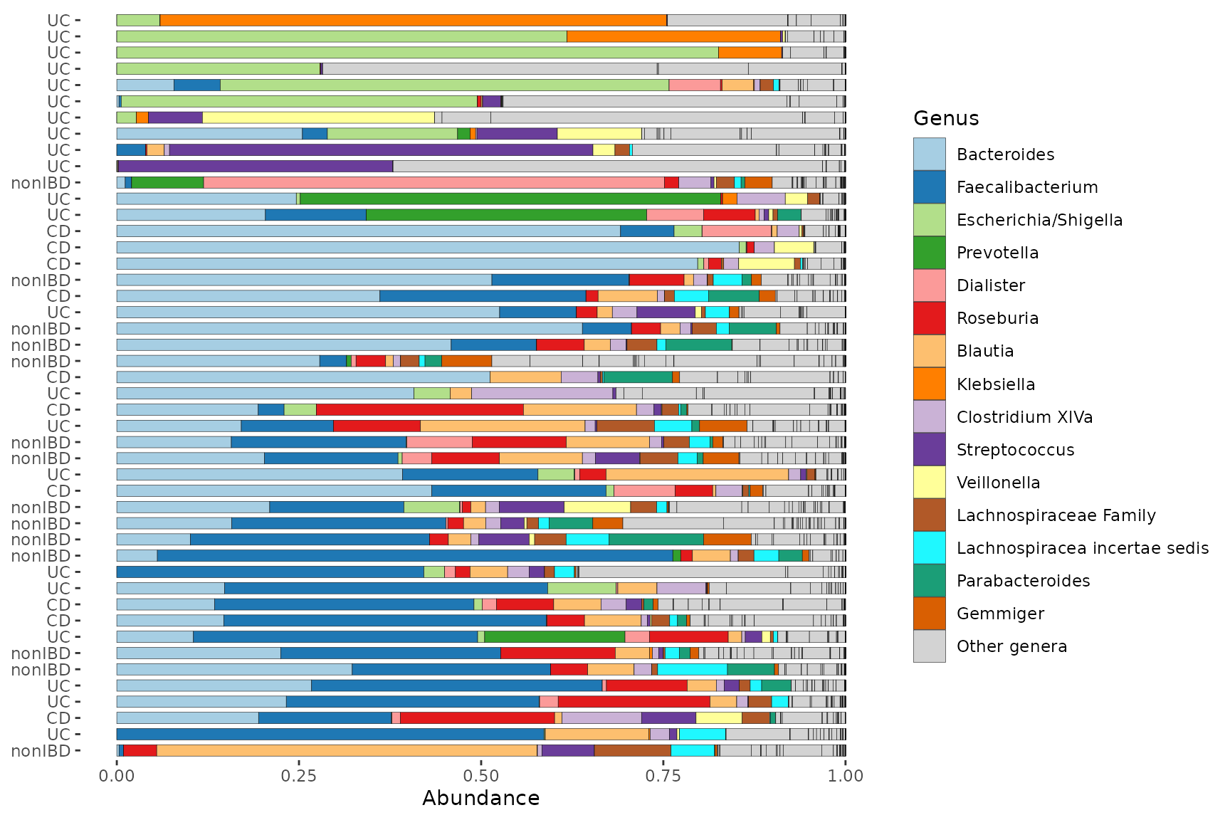
Figure from the microbiomeViz documentation (Barnett, Arts, and Penders 2021).

Focus-plus-Context: Barplots

Stacked barplots visualize sample-to-sample variation in microbiome community structure. They struggle to show finer taxonomic resolutions.

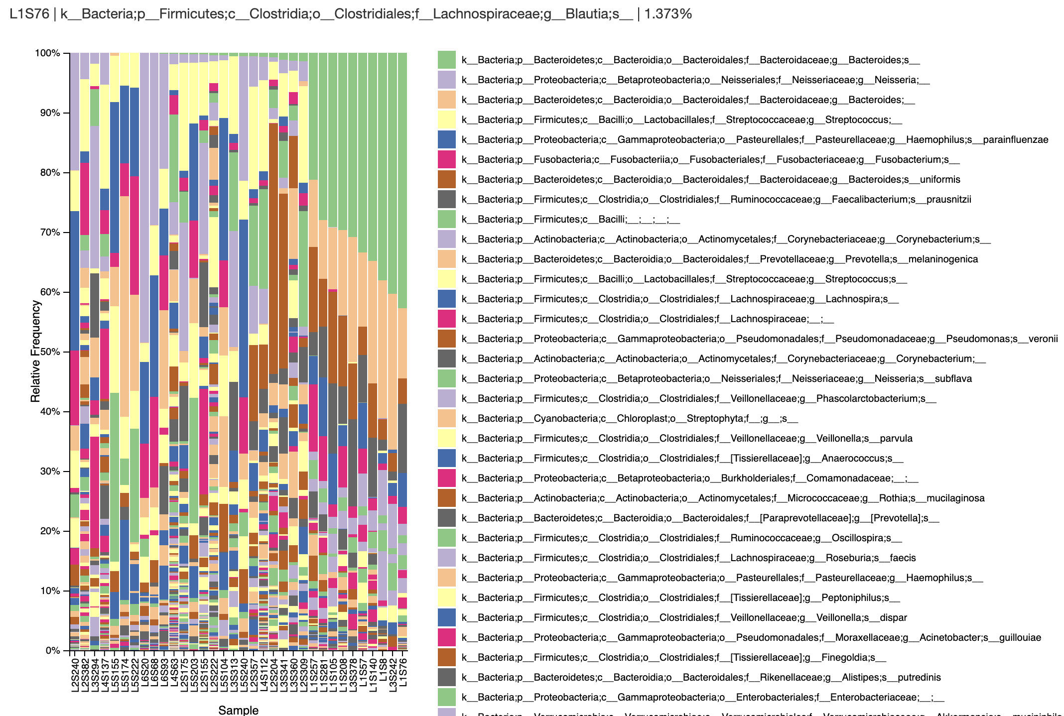
Figure from the Qiime2 View documentation (Bolyen et al. 2019).

Phylobar

Applying focus-plus-context reveals rare taxa abundances while preserving overall structure

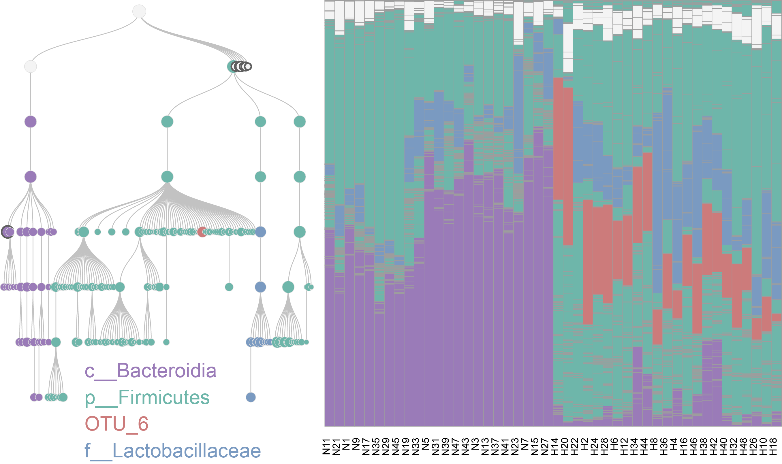
Figure from the phylobar documentation (Kuo et al. 2025).

Mammoth

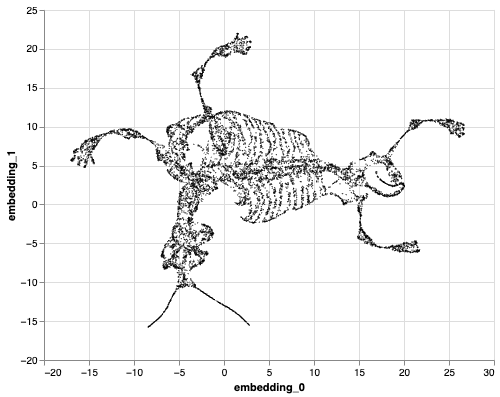
This example comes from (“Understanding UMAP — Pair-Code.github.io”; Noichl). The 3D skeleton scans were produced by the Smithsonian, and we can use nonlinear dimensionality reduction to “flatten” the skeleton into 2D.

Mammoth

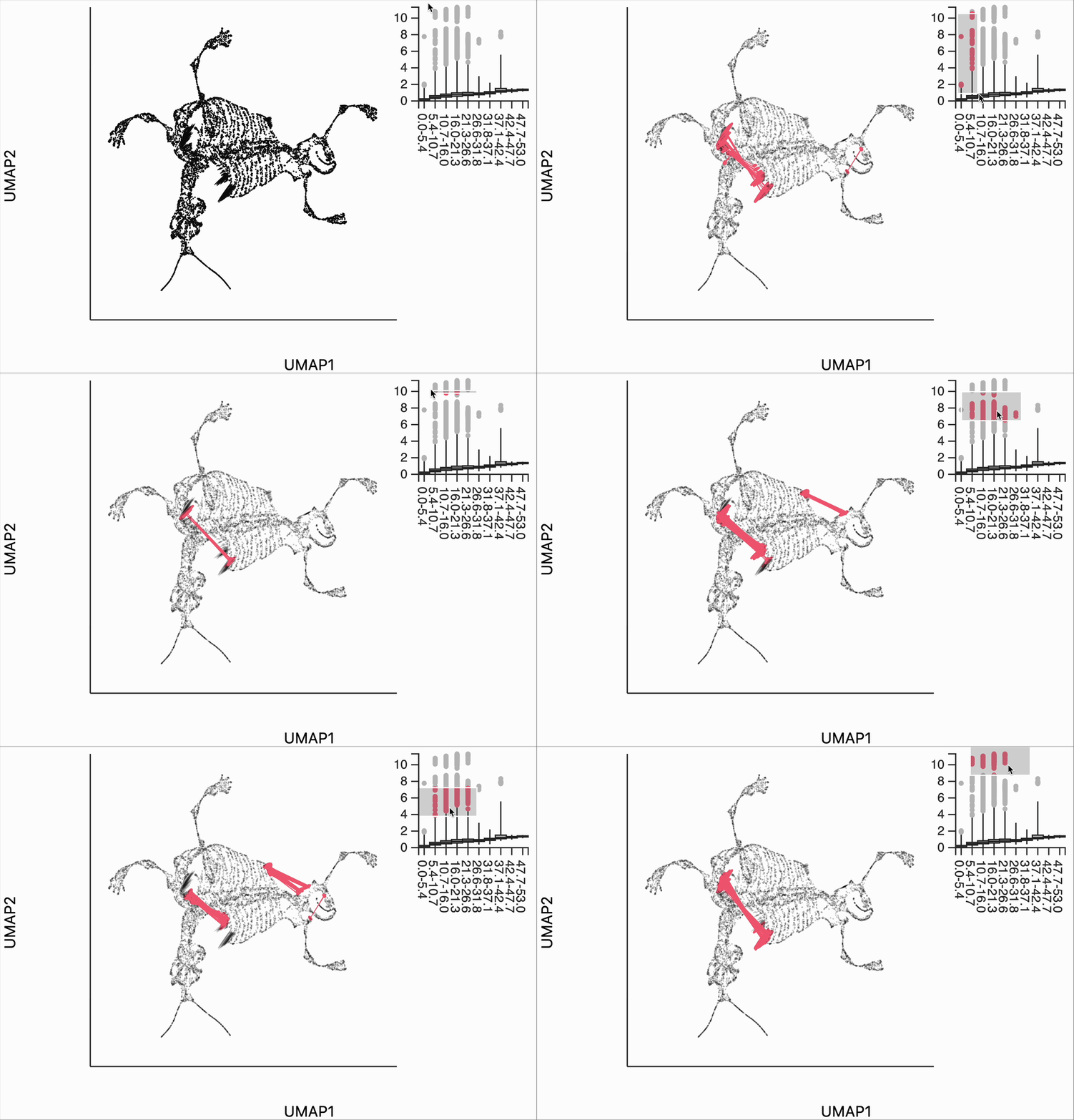
This is the embedding when applying UMAP with a 50 nearest-neighbor graph and min_dist = 0.5.

Mammoth

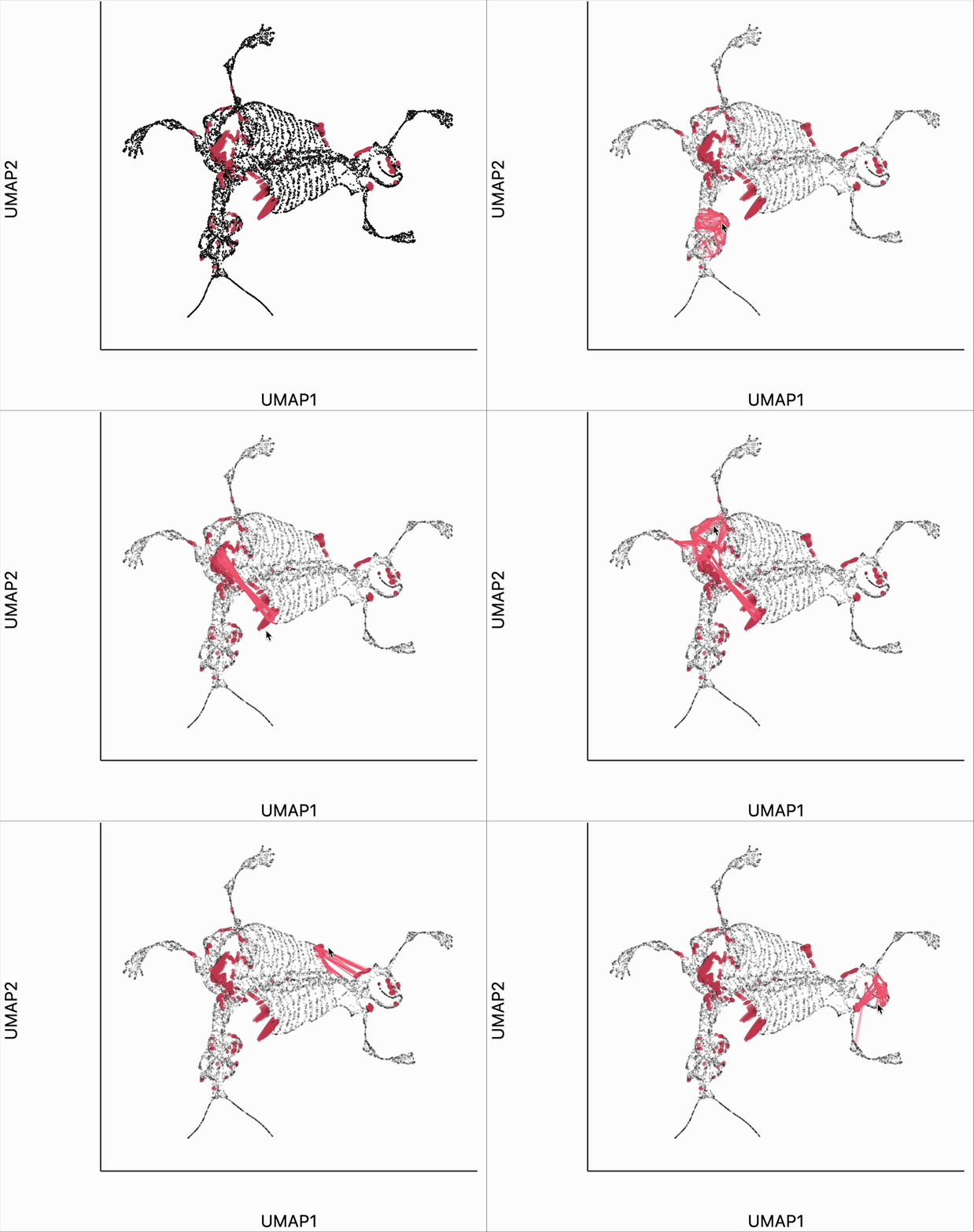
Parts of the shoulders, head, and tail are further apart in the embedding compared to the original data. Most other distortions are points that are placed too close to one another.

Mammoth

Parts of the shoulders, head, and tail are further apart in the embedding compared to the original data. Most other distortions are points that are placed too close to one another.

Graph Laplacian

To compute \(L\), we use the estimator from (Coifman and Lafon 2006).

1. Build the kernel matrix \(W_{kl} = \exp(-\|X_k - X_l\|^2 / h)\), where \(h\) is a bandwidth hyperparameter.

2. Normalize both columns and rows. \[\begin{align*} D &= \text{diag}(W\mathbf{1}) \qquad \tilde{W} = D^{-1}WD^{-1} \\ \tilde{D} &= \text{diag}(\tilde{W}\mathbf{1}) \qquad L = \tilde{D}^{-1}\tilde{W} \end{align*}\] Column normalization accounts for differences in sampling density.

Pushforward Metric

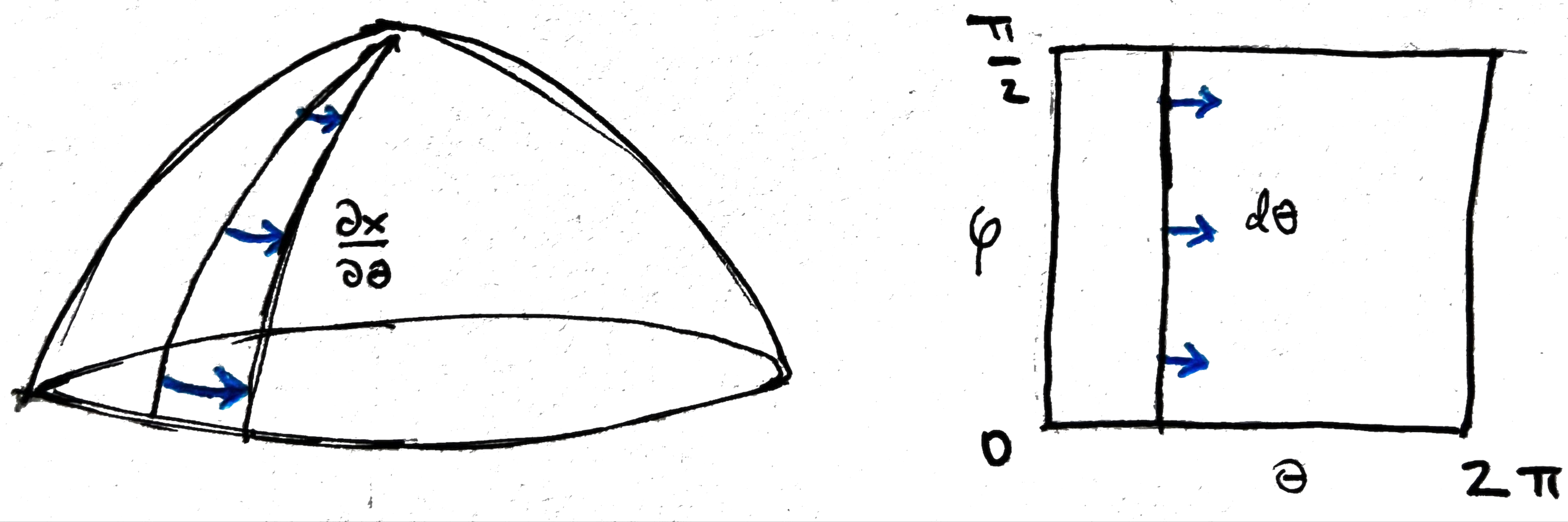
What does a small step in the embedding space correspond to in \(\mathcal{M}\)? The pushforward metric answers this,

\[\begin{align*} g_{ij} = \left\langle \frac{\partial\mathbf{x}}{\partial z^i}, \frac{\partial\mathbf{x}}{\partial z^j}\right\rangle_{\mathbb{R}^3} \end{align*}\]

This varies across \(p \in \mathcal{M}\) but we suppress it from the notation.

Pushforward Metric

In the sphere example, these derivatives can be directly computed and to obtain,

\[\begin{align*} G = \begin{pmatrix} \cos^2\varphi & 0 \\ 0 & 1 \end{pmatrix} \end{align*}\] Near the equator (\(\varphi \approx 0\)), a small step in \(\theta\) covers more distance than near the north pole (\(\varphi \approx \frac{\pi}{2}\)).

Derivation of \(G\)

First note that, \[\begin{align*} \frac{\partial\mathbf{x}}{\partial \theta} = \left(-\cos\varphi\sin\theta, \cos\varphi\cos\theta, 0\right). \end{align*}\] Therefore, \[\begin{align*} g_{11} &= \left\langle \frac{\partial\mathbf{x}}{\partial \theta}, \frac{\partial\mathbf{x}}{\partial \theta}\right\rangle_{\mathbb{R}^3} \\ &= \cos^2\varphi\sin^2\theta + \cos^2\varphi\cos^2\theta \\ &= \cos^2\varphi \end{align*}\]

Derivation of \(H\) from \(\Delta\left(fg\right)\)

By the product formula with \(z^1 = \theta\): \[\begin{align*} h^{11} = \langle \nabla \theta, \nabla \theta \rangle_{g_0} = \frac{1}{2}\left[\Delta(\theta^2) - 2\theta\Delta\theta\right] \end{align*}\]

Derivation of \(H\) from \(\Delta\left(fg\right)\)

The general formula for the Laplace-Beltrami operator is \[\Delta f = \frac{1}{\sqrt{\det G}}\sum_{i,j}\frac{\partial}{\partial z^i}\left(\sqrt{\det G}\, g^{ij}\frac{\partial f}{\partial z^j}\right).\]

Since \(\det(G) = \cos^2\varphi\) and the off-diagonal \(g^{ij}\) are zero, \[\begin{align*} \Delta f = \frac{1}{\cos^2\varphi}\frac{\partial^2 f}{\partial\theta^2} + \frac{1}{\cos\varphi}\frac{\partial}{\partial\varphi}\left(\cos\varphi\frac{\partial f}{\partial\varphi}\right) \end{align*}\]

Derivation of \(H\) from \(\Delta\left(fg\right)\)

We can plug in the choices of \(f\) that we care about, \[\begin{align*} \Delta\theta &= 0\\ \Delta(\theta^2) &= \frac{1}{\cos^2\varphi}\frac{\partial^2(\theta^2)}{\partial\theta^2} = \frac{2}{\cos^2\varphi} \end{align*}\]

and then substitute into the formula from 2 slides ago, \[\begin{align*} h^{11} = \frac{1}{2}\left[\frac{2}{\cos^2\varphi} - 2\theta \cdot 0\right] = \frac{1}{\cos^2\varphi}. \end{align*}\]

Interaction Gulfs

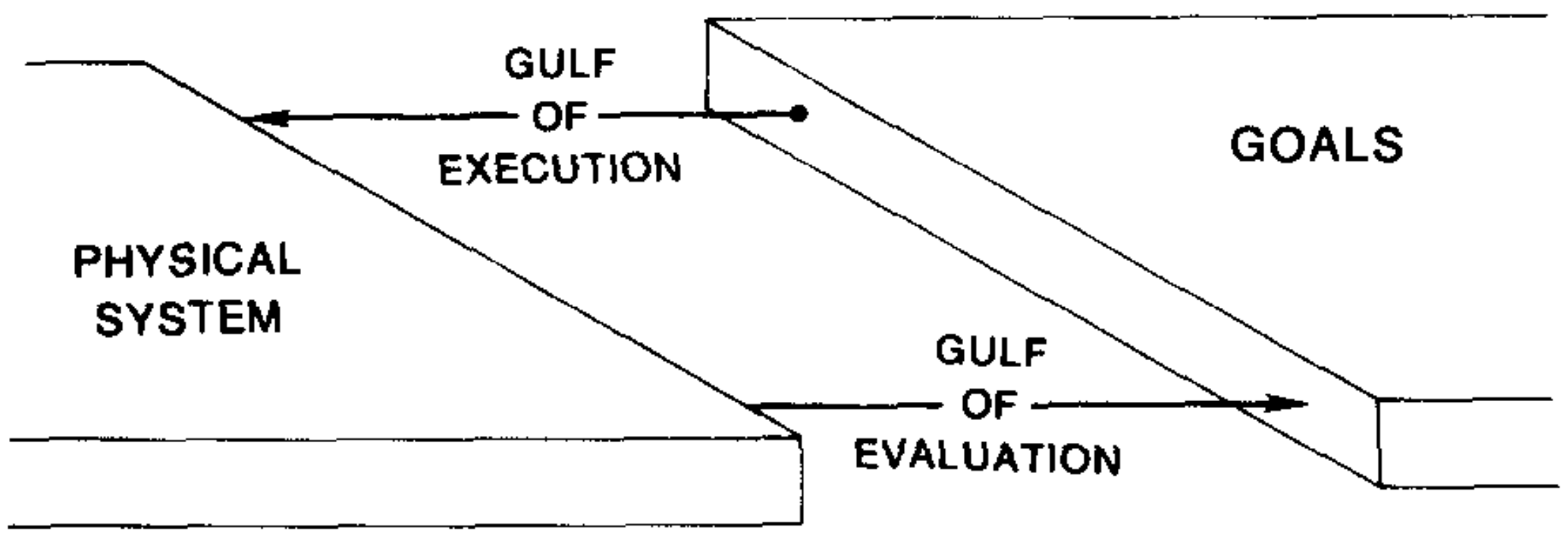
There are two classic challenges in interactive interfaces (Hutchins, Hollan, and Norman 1985),

• Gulf of Execution: The gap between what you want to do and how you specify it in the system.

These challenges also apply to interactive data analysis.

Interaction Gulfs

There are two classic challenges in interactive interfaces (Hutchins, Hollan, and Norman 1985),

• Gulf of Evaluation: The gap between what the system shows you and an understanding of what it represents.

These challenges also apply to interactive data analysis.

Specious Art

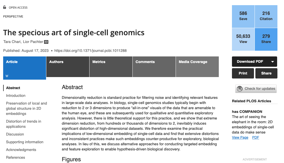
Nonlinear dimensionality reduction has become the source of widespread concern in the single-cell literature (Chari and Pachter 2023).

Dual Pushforward Metric

Alternatively, the gradients \(\nabla z^i\) of the embedding dimensions also reflect distortion.

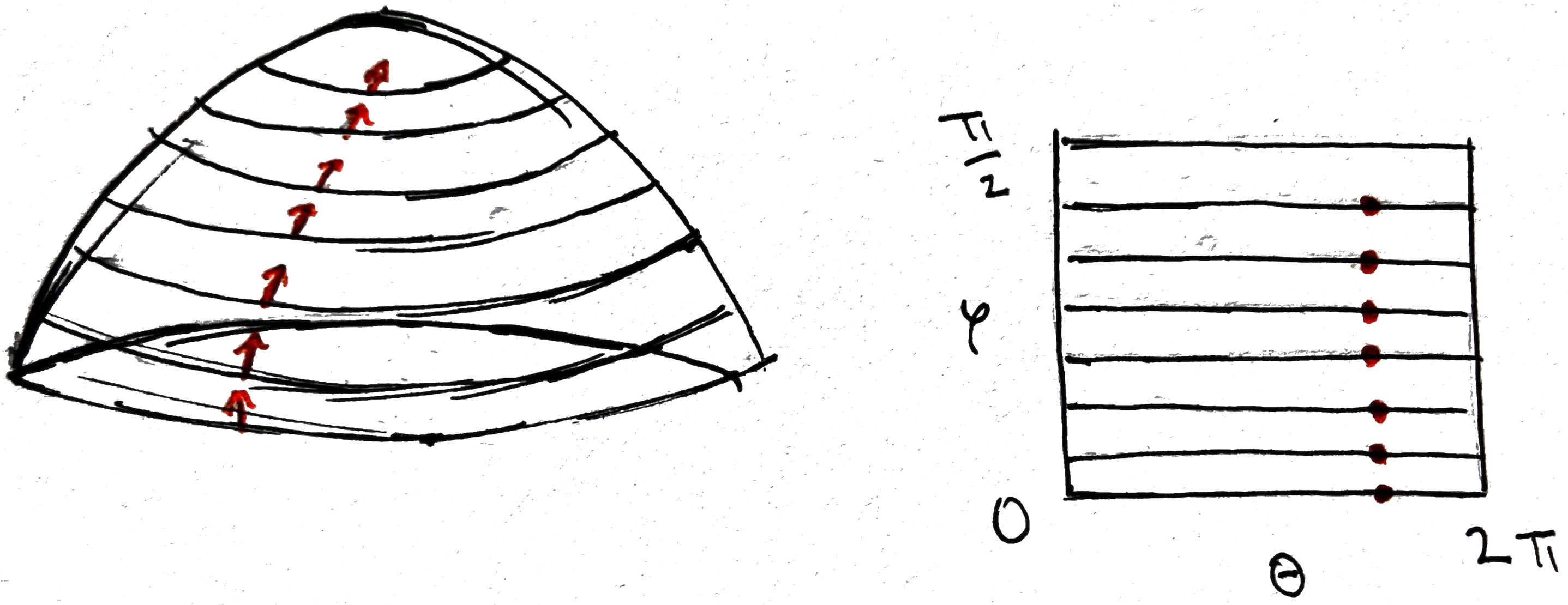
In contrast, the gradients \(\nabla z^{\varphi}\) don’t depend on \(\varphi\).

Comparison with LOO-map

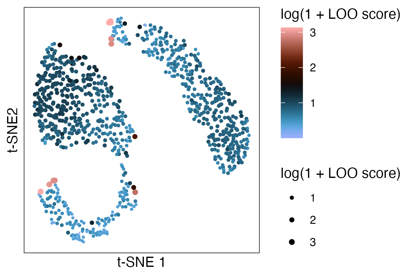
The stability-based algorithm (Liu, Ma, and Zhong 2025) gives a similar interpretation. But the visual encoding is more subtle, and the leave-one-out approach is time consuming even with approximations.

Distortions in \(t\)-SNE and UMAP

They can make high-dimensional random walks look artificially smooth…

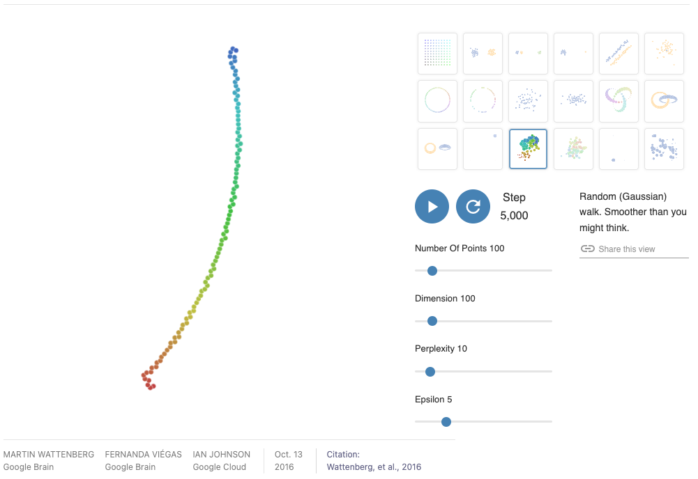Example from (Wattenberg, Viégas, and Johnson 2016).

Hydra Cell Atlas

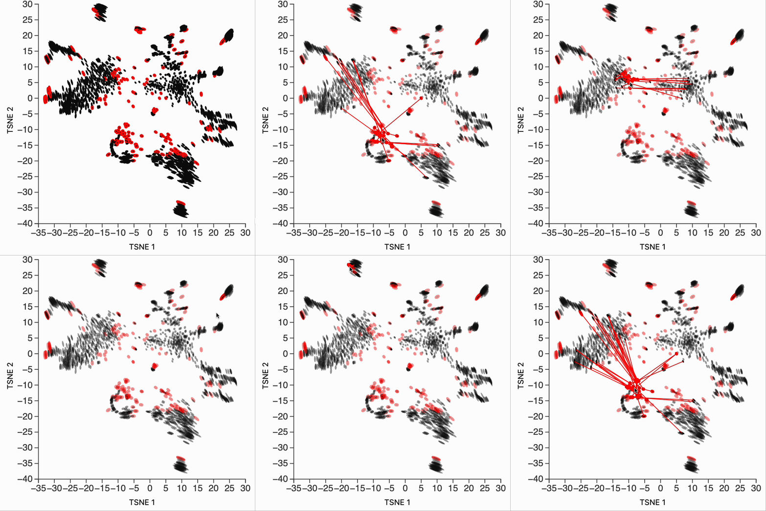
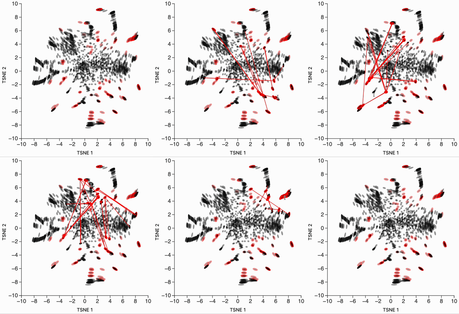
In this hydra cell differentiation dataset (Siebert et al. 2019; Xia, Lee, and Li 2024), \(t\)-SNE (perplexity = 80) collapses points along the dataset periphery and exaggerates between-cluster distances

Hydra Cell Atlas

At perplexity = 500, the clusters are more reliable, but peripheral samples are in fact closer than they appear

Hydra Cell Atlas

The local isometry visualization highlights some “threads” are more spread in the original data.

References

Barnett, David J. M., Ilja C. W. Arts, and John Penders. 2021. “microViz: An r Package for Microbiome Data Visualization and Statistics.” Journal of Open Source Software 6 (63): 3201. https://doi.org/10.21105/joss.03201.

Bolyen, Evan, Jai Ram Rideout, Matthew R. Dillon, Nicholas A. Bokulich, Christian C. Abnet, Gabriel A. Al-Ghalith, Harriet Alexander, et al. 2019. “Reproducible, Interactive, Scalable and Extensible Microbiome Data Science Using QIIME 2.” Nature Biotechnology 37 (8): 852–57. https://doi.org/10.1038/s41587-019-0209-9.

Chari, Tara, and Lior Pachter. 2023. “The Specious Art of Single-Cell Genomics.” Edited by Jason A. Papin. PLOS Computational Biology 19 (8): e1011288. https://doi.org/10.1371/journal.pcbi.1011288.

Coifman, Ronald R., and Stéphane Lafon. 2006. “Diffusion Maps.” Applied and Computational Harmonic Analysis 21 (1): 5–30. https://doi.org/10.1016/j.acha.2006.04.006.

Heer, Jeffrey, and Stuart K. Card. 2004. “DOITrees Revisited: Scalable, Space-Constrained Visualization of Hierarchical Data.” In Proceedings of the Working Conference on Advanced Visual Interfaces, 421–24. AVI ’04. New York, NY, USA: Association for Computing Machinery. https://doi.org/10.1145/989863.989941.

Hein, Matthias, Jean-Yves Audibert, and Ulrike von Luxburg. 2005. “From Graphs to Manifolds – Weak and Strong Pointwise Consistency of Graph Laplacians.” In Learning Theory, 470–85. Springer Berlin Heidelberg. https://doi.org/10.1007/11503415_32.

Hutchins, Edwin L., James D. Hollan, and Donald A. Norman. 1985. “Direct Manipulation Interfaces.” Human–Computer Interaction 1 (4): 311–38. https://doi.org/10.1207/s15327051hci0104_2.

Kobak, Dmitry, and George C. Linderman. 2021. “Initialization Is Critical for Preserving Global Data Structure in Both t-SNE and UMAP.” Nature Biotechnology 39 (2): 156–57. https://doi.org/10.1038/s41587-020-00809-z.

Kuo, Megan, Kim-Anh Lê Cao, Saritha Kodikara, Jiadong Mao, and Kris Sankaran. 2025. “Phylobar: An r Package for Multiresolution Compositional Barplots in Omics Studies,” November. https://doi.org/10.1101/2025.11.05.686662.

Laskowski, Piotr H. 1989. “The Traditional and Modern Look at Tissot’s Indicatrix.” The American Cartographer 16 (2): 123–33.

Liu, Zhexuan, Rong Ma, and Yiqiao Zhong. 2025. “Assessing and Improving Reliability of Neighbor Embedding Methods: A Map-Continuity Perspective.” Nature Communications 16 (1). https://doi.org/10.1038/s41467-025-60434-9.

McQueen, James, Marina Meilă, Jacob VanderPlas, and Zhongyue Zhang. 2016. “Megaman: Scalable Manifold Learning in Python.” Journal of Machine Learning Research 17 (148): 1–5.

References (cont.)

Narayan, Ashwin, Bonnie Berger, and Hyunghoon Cho. 2021. “Assessing Single-Cell Transcriptomic Variability Through Density-Preserving Data Visualization.” Nature Biotechnology 39 (6): 765–74.

Noichl, Max. “Max Noichl | Flattening Mammoths — Maxnoichl.eu.” https://www.maxnoichl.eu/projects/mammoth/.

Packer, Jonathan S., Qin Zhu, Chau Huynh, Priya Sivaramakrishnan, Elicia Preston, Hannah Dueck, Derek Stefanik, et al. 2019. “A Lineage-Resolved Molecular Atlas of c. Elegans Embryogenesis at Single-Cell Resolution.” Science 365 (6459). https://doi.org/10.1126/science.aax1971.

Perrault-Joncas, Dominique, and Marina Meila. 2006. “Metric Learning of Manifolds.” Semisupervised Learn 1: 293–306.

Siebert, Stefan, Jeffrey A. Farrell, Jack F. Cazet, Yashodara Abeykoon, Abby S. Primack, Christine E. Schnitzler, and Celina E. Juliano. 2019. “Stem Cell Differentiation Trajectories in Hydra Resolved at Single-Cell Resolution.” Science 365 (6451). https://doi.org/10.1126/science.aav9314.

“Understanding UMAP — Pair-Code.github.io.” https://pair-code.github.io/understanding-umap/.

Venna, Jarkko, and Samuel Kaski. 2006. “Local Multidimensional Scaling.” Neural Networks 19 (6–7): 889–99. https://doi.org/10.1016/j.neunet.2006.05.014.

Wattenberg, Martin, Fernanda Viégas, and Ian Johnson. 2016. “How to Use t-SNE Effectively.” Distill. https://doi.org/10.23915/distill.00002.

Wolf, F. Alexander, Philipp Angerer, and Fabian J. Theis. 2018. “SCANPY: Large-Scale Single-Cell Gene Expression Data Analysis.” Genome Biology 19 (1). https://doi.org/10.1186/s13059-017-1382-0.

Xia, Lucy, Christy Lee, and Jingyi Jessica Li. 2024. “Statistical Method scDEED for Detecting Dubious 2D Single-Cell Embeddings and Optimizing t-SNE and UMAP Hyperparameters.” Nature Communications 15 (1): 1753.