\def\absarg#1{\left|#1\right|} \def\Earg#1{\mathbf{E}\left[#1\right]} \def\reals{\mathbb{R}} % Real number symbol \def\integers{\mathbb{Z}} % Integer symbol \def\*#1{\mathbf{#1}} \def\m#1{\boldsymbol{#1}} \def\FDR{\widehat{\operatorname{FDR}}} \def\Gsn{\mathcal{N}} \def\Unif{\operatorname{Unif}} \def\Bern{\operatorname{Bern}}
Kris Sankaran
14 | July | 2023
https://github.io/krisrs1128/LSLab
Code: https://go.wisc.edu/s8hdtt
Examples
- Microbiome: Is taxon m associated with the development of autism in infants?
- Epigenetics: Is CpG site m differentially methlyated among smokers?
- Cancer: Is elevated immune cell expression of gene m associated with improved survival rates?
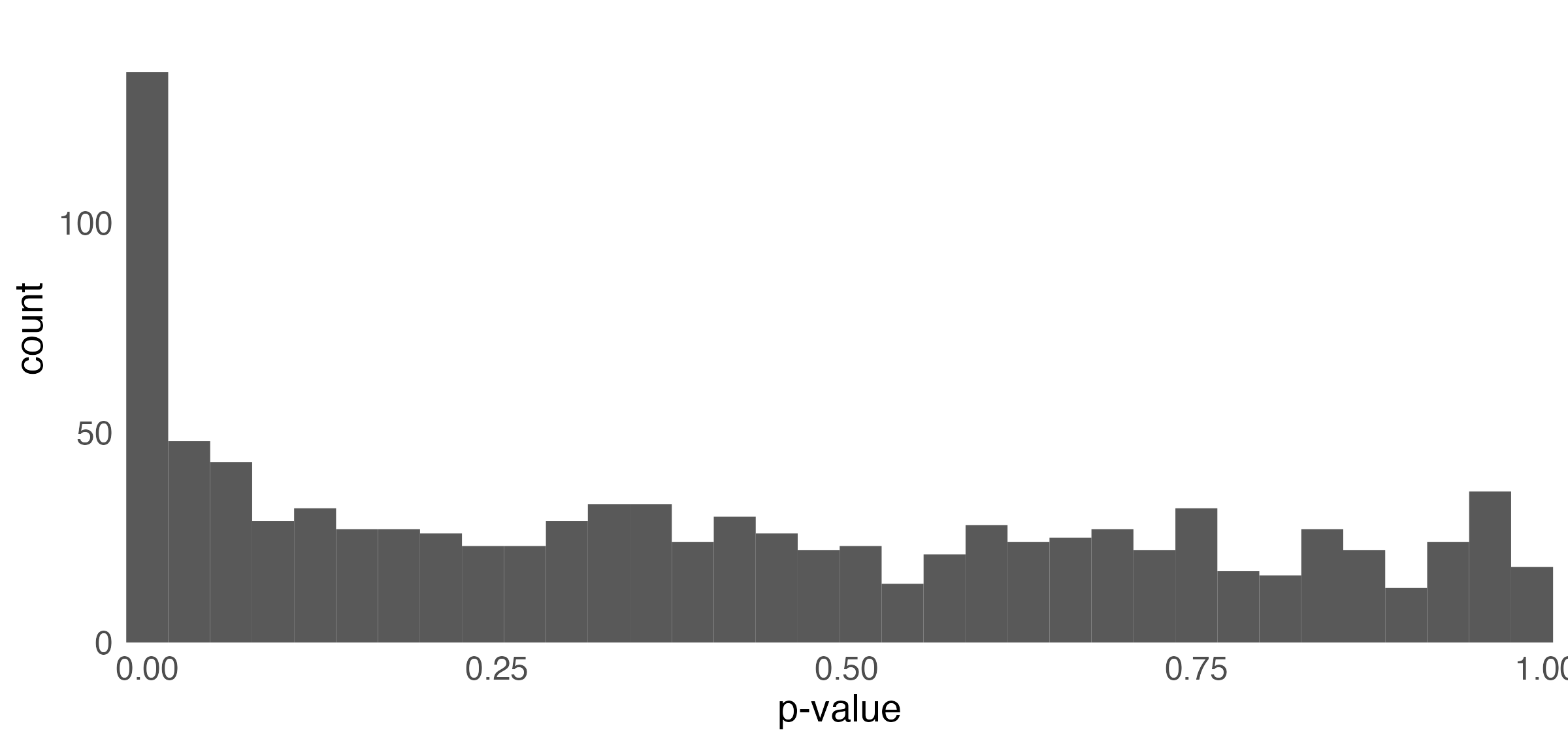
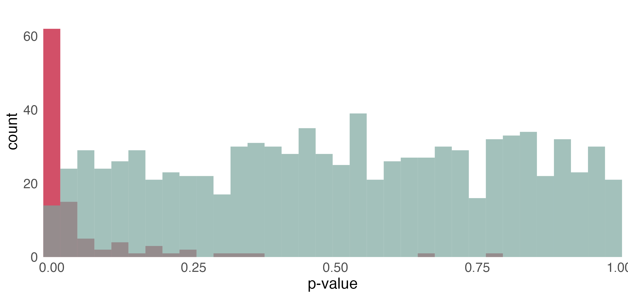
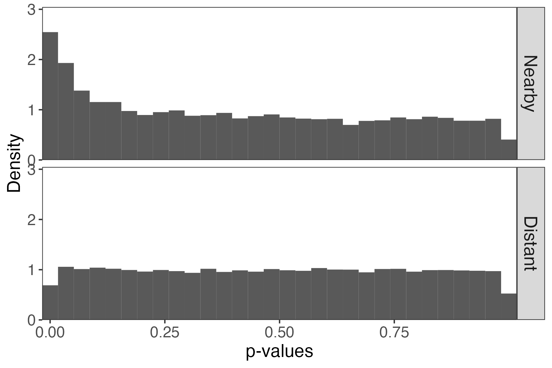
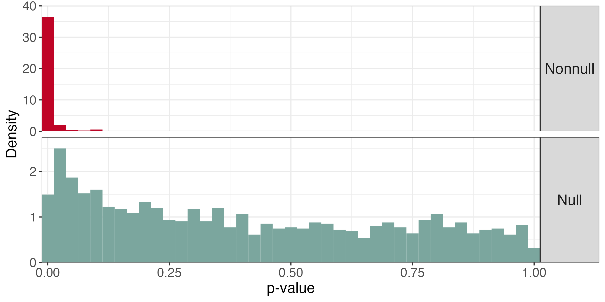
p-value histogram
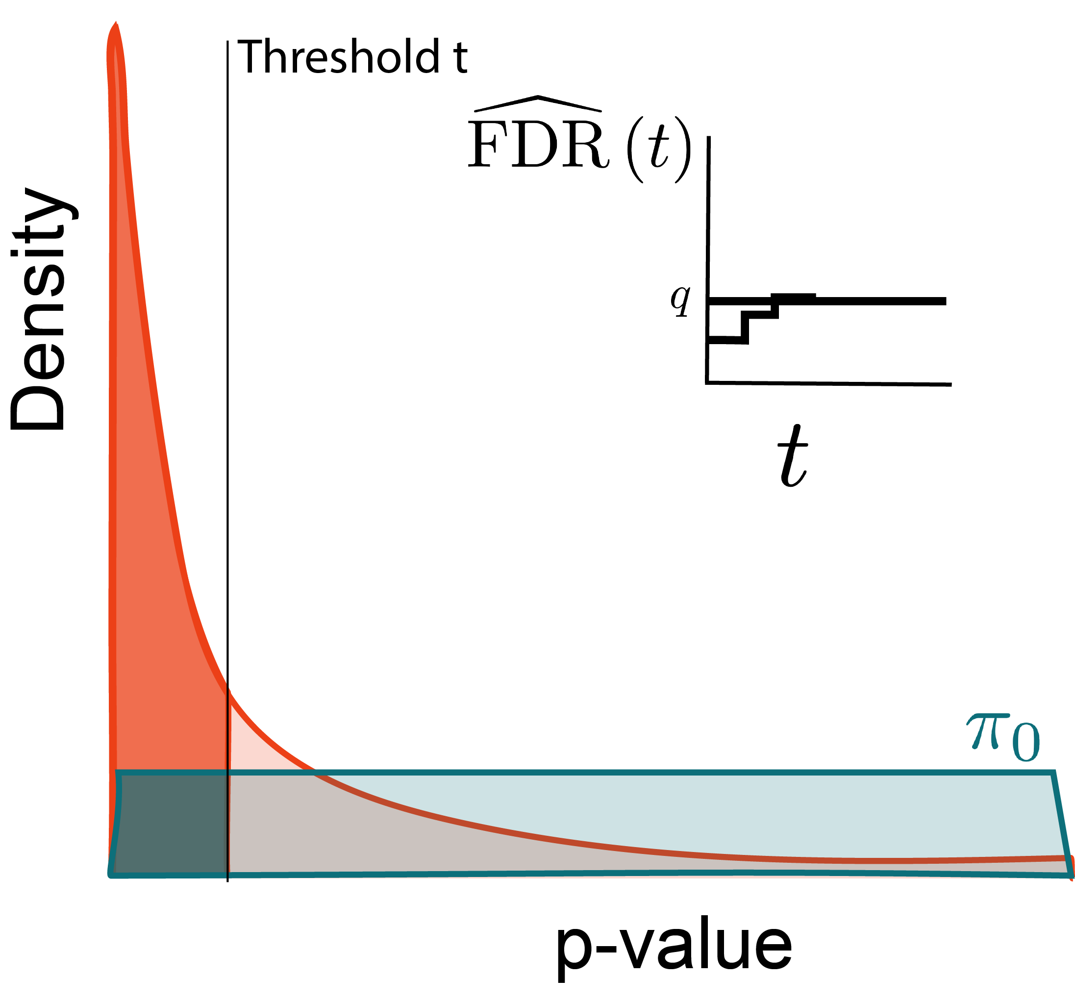
- Under the null, the p-values follow a uniform distribution.
- The spike near 0 \implies true alternative hypotheses
- \pi_{0} refers to the true proportion of nulls
p-value histogram
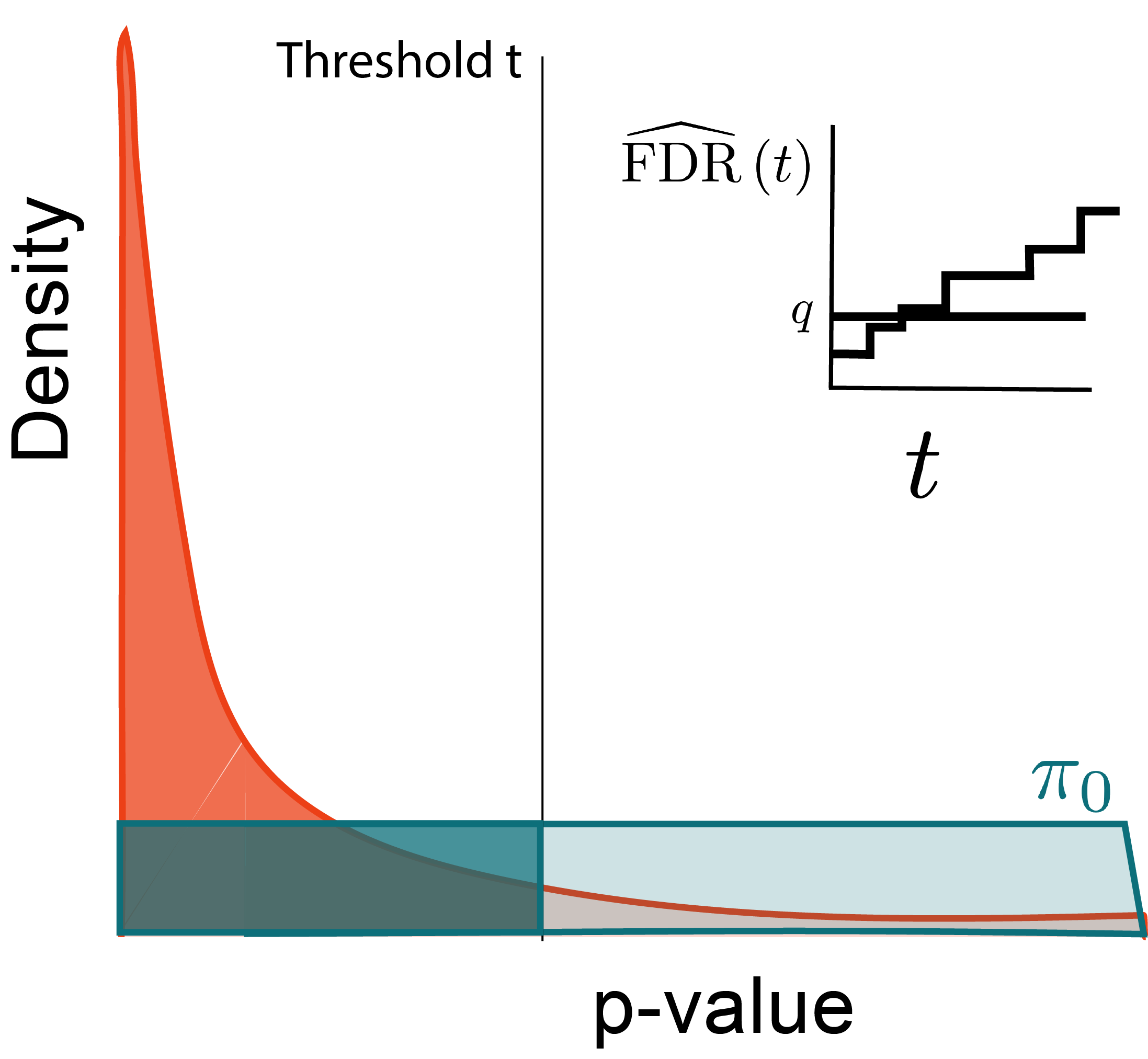
- Under the null, the p-values follow a uniform distribution.
- The spike near 0 \implies true alternative hypotheses
- \pi_{0} refers to the true proportion of nulls
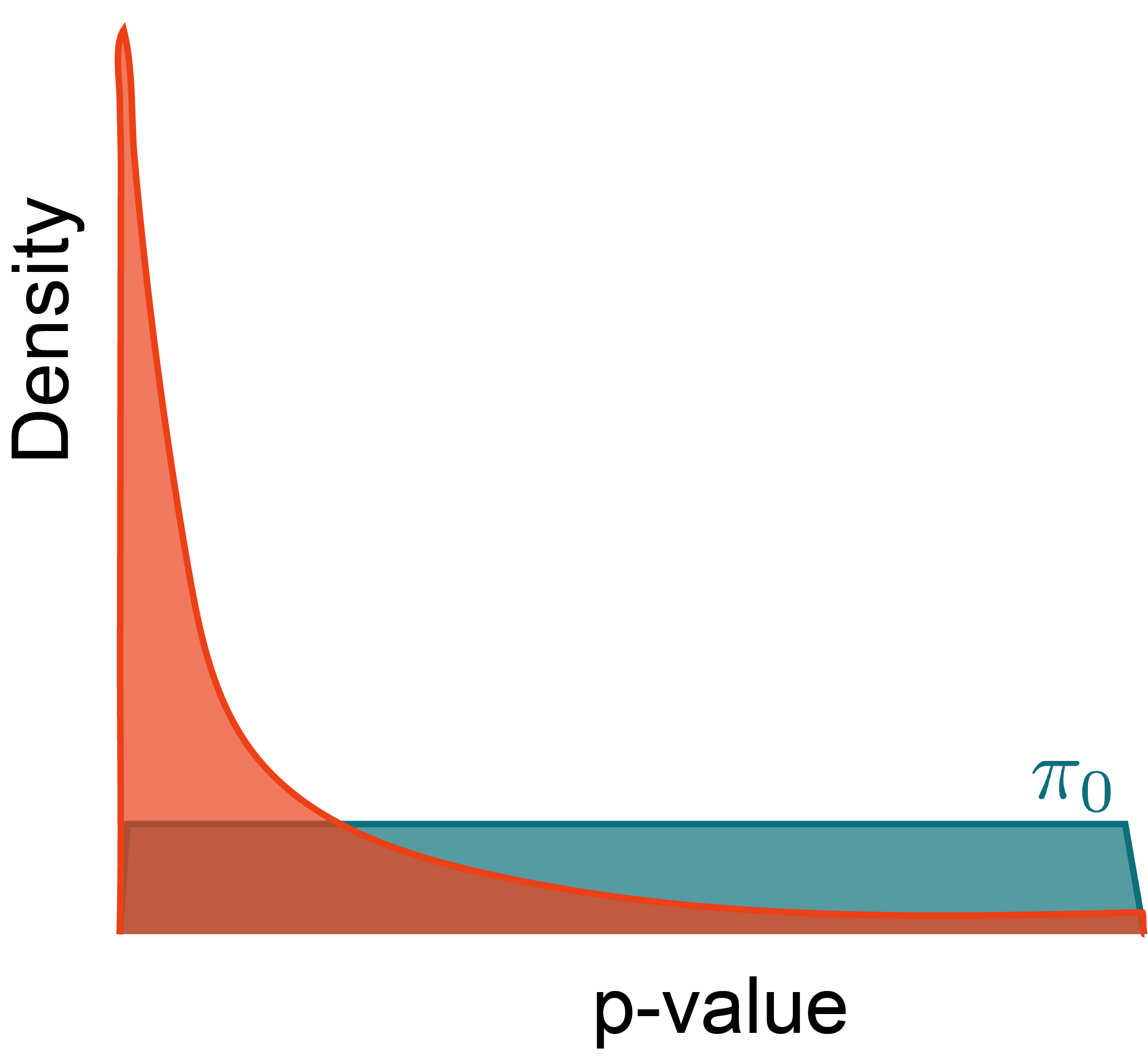
p-value histogram
- Under the null, the p-values follow a uniform distribution.
- The spike near 0 \implies true alternative hypotheses
- \pi_{0} refers to the true proportion of nulls
Why?
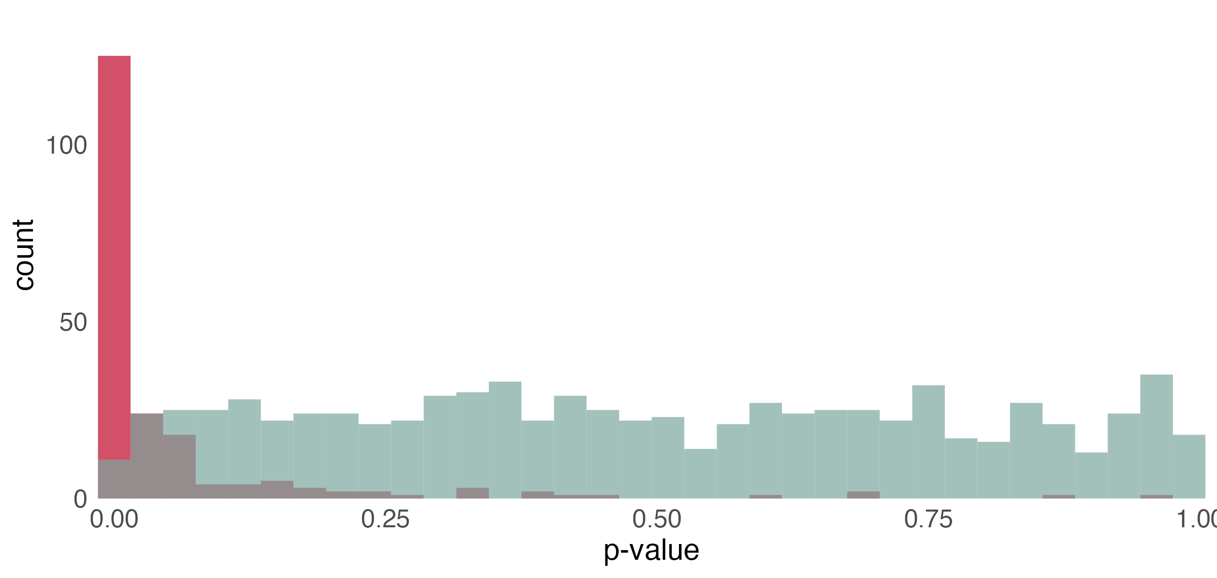
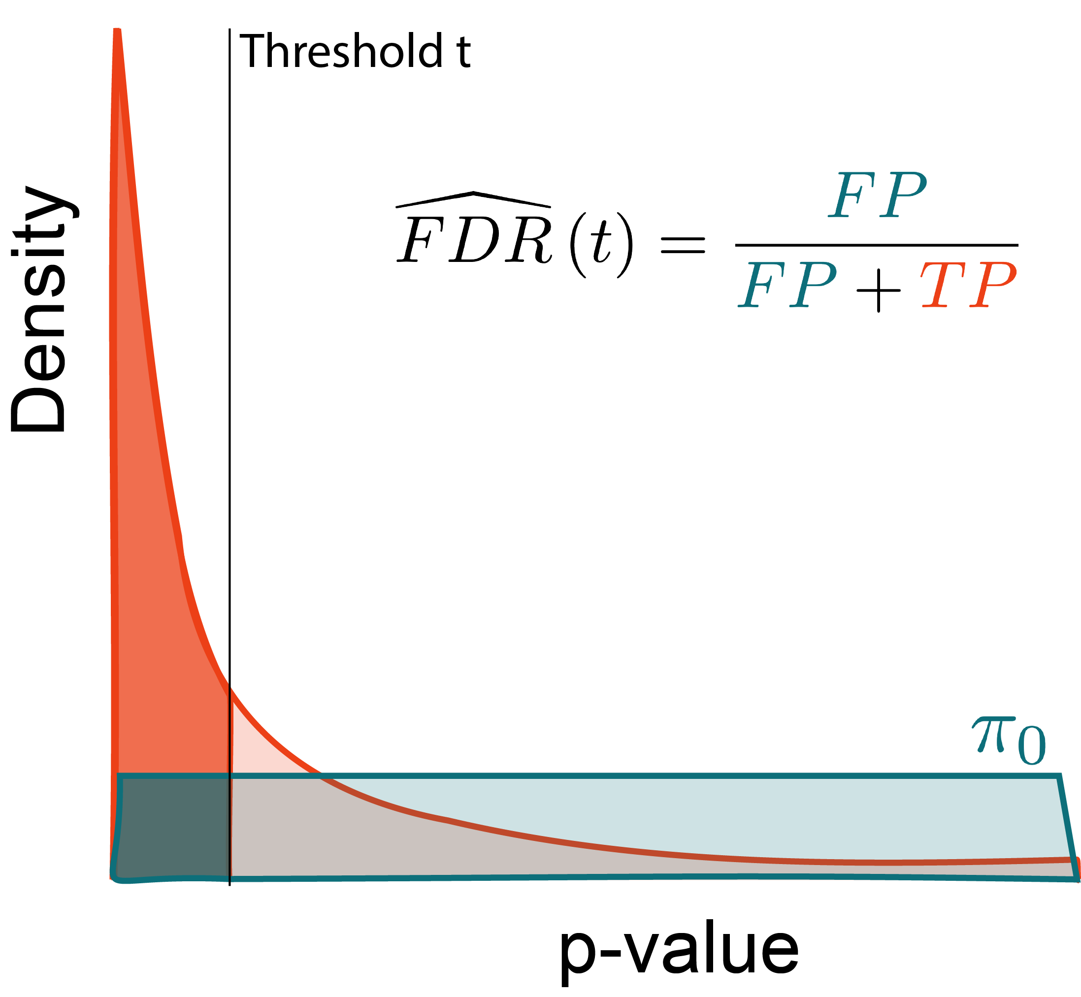
At any threshold t, estimate the FDR using relative areas from the null and alternative densities.
Why?
At any threshold t, estimate the FDR using relative areas from the null and alternative densities.
Why?
Let R\left(t\right) be the number of rejected hypotheses at threshold t. Then,
\begin{align*} \FDR\left(t\right) &= \frac{\pi_{0}Mt}{R\left(t\right)} \end{align*}
Why?
Maximize the number of rejections while limiting false discoveries.
Optimize: \begin{align*} \text{maximize } &R\left(t\right) \\ \text{subject to } &\FDR\left(t\right) \leq q \end{align*}
Why?
Maximize the number of rejections while limiting false discoveries.
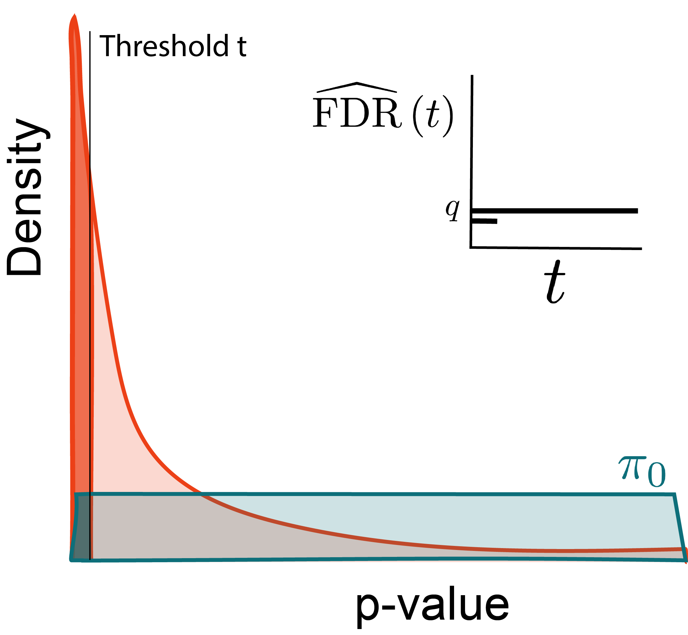
Optimize: \begin{align*} \text{maximize } &t \\ \text{subject to } &\FDR\left(t\right) \leq q \end{align*}
Why?
Larger thresholds let more hypotheses through.
Optimize: \begin{align*} \text{maximize } & t \\ \text{subject to } &\FDR\left(t\right) \leq q \end{align*}
Why?
Larger thresholds let more hypotheses through.
Optimize: \begin{align*} \text{maximize } & t \\ \text{subject to } &\FDR\left(t\right) \leq q \end{align*}
Why?
Larger thresholds let more hypotheses through.
Optimize: \begin{align*} \text{maximize } &t \\ \text{subject to } &\FDR\left(t\right) \leq q \end{align*}
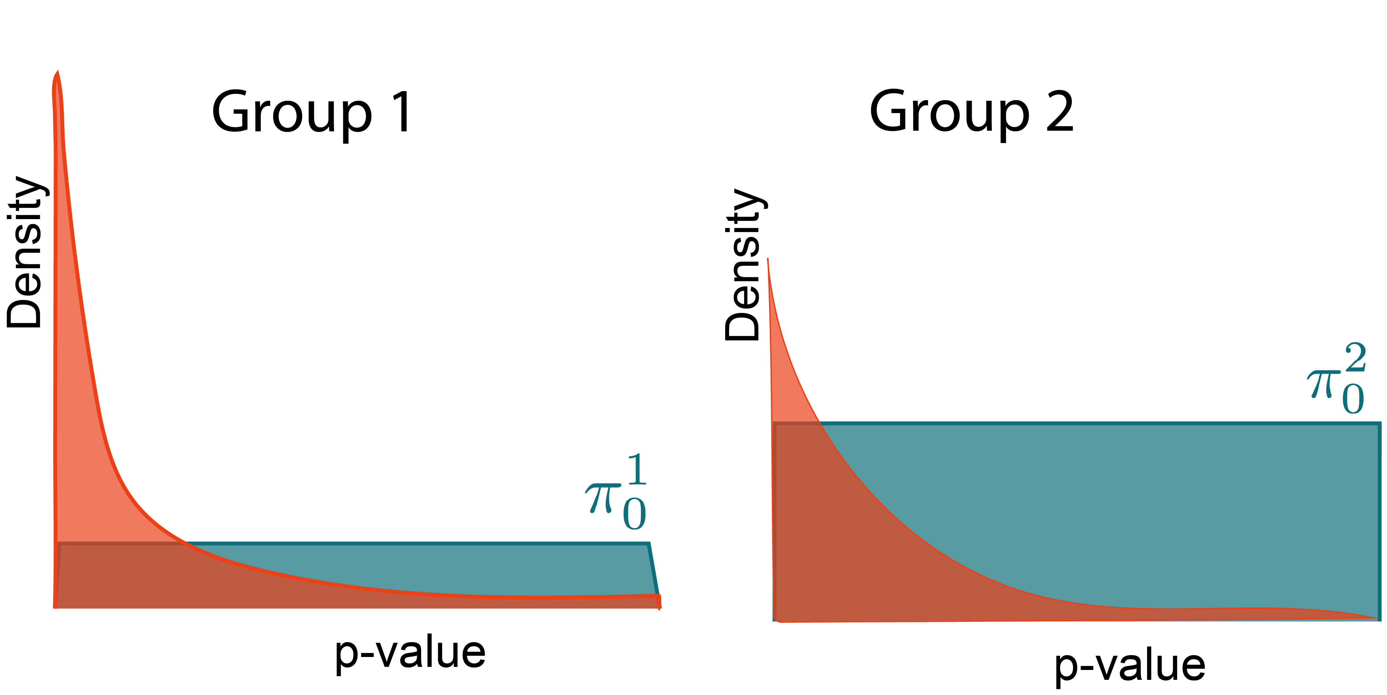
Hypotheses are not identical
- We may know in advance that some hypotheses are more likely to be rejected than others.
- Prior literature
- Number of mapped reads
- This information can improve power. We'll discuss [2], but see [3; 4; 5; 6]
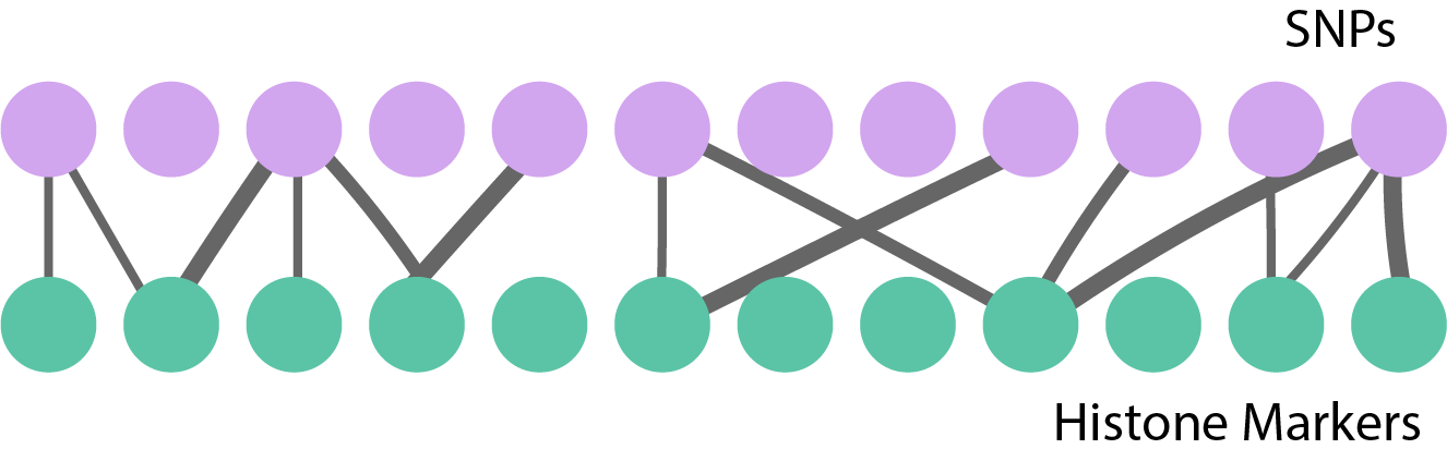
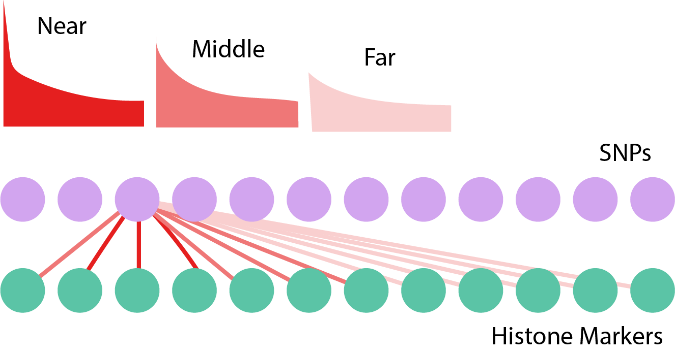
Example: Testing Pairs
Suppose we are testing associations between,
- SNPs x_{1}, \dots, x_{I}
- Histone Markers y_{1}, \dots, y_{J}
H_{m}: \text{Cor}\left(x_{i}, y_{j}\right) = 0.
Even for moderate I, J, this is many tests!
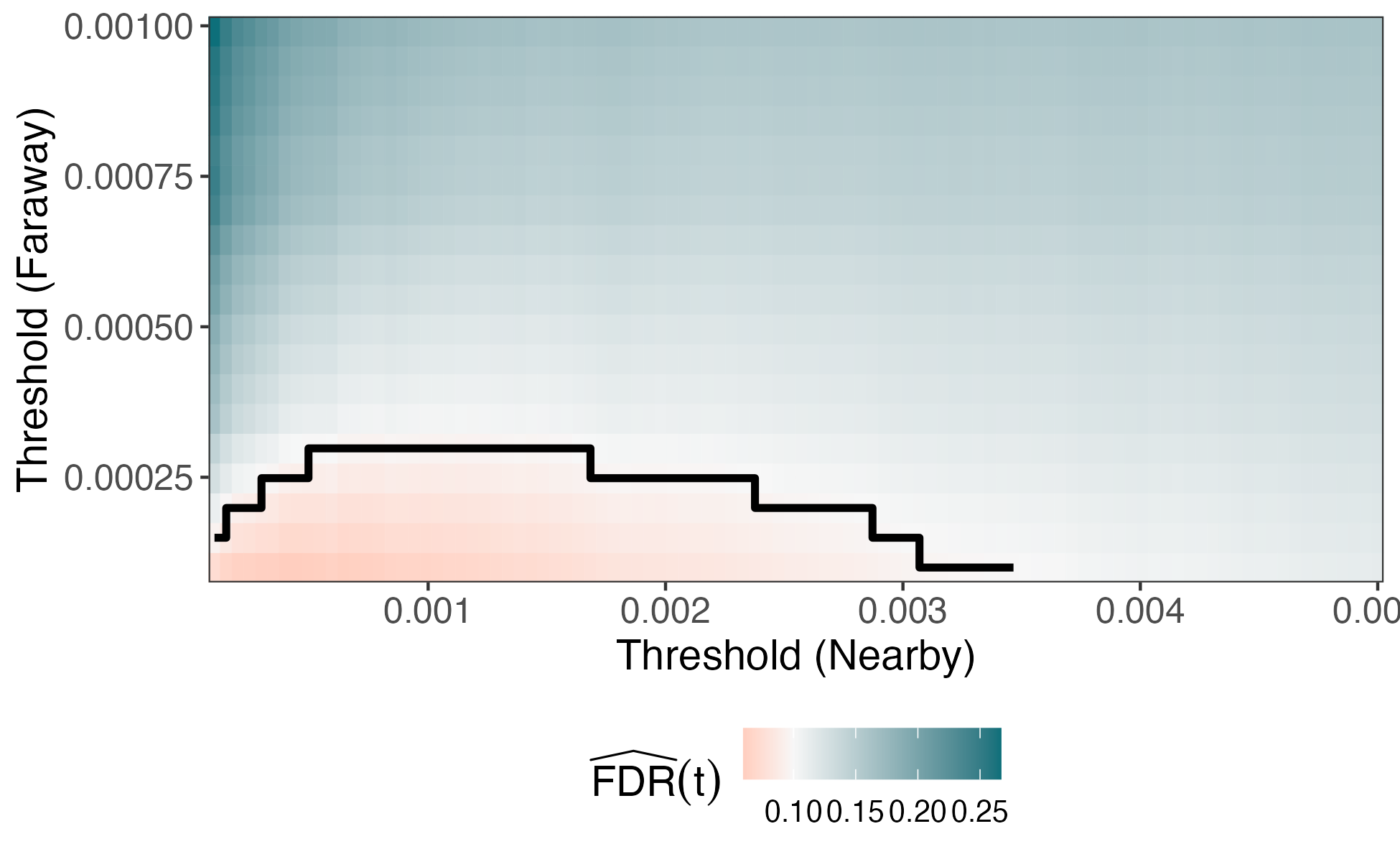
Grouping by Distance
- Group the distances into bins 1, \dots, G.
- We use different thresholds \*t = \left(t_{1}, \dots, t_{G}\right) across groups.
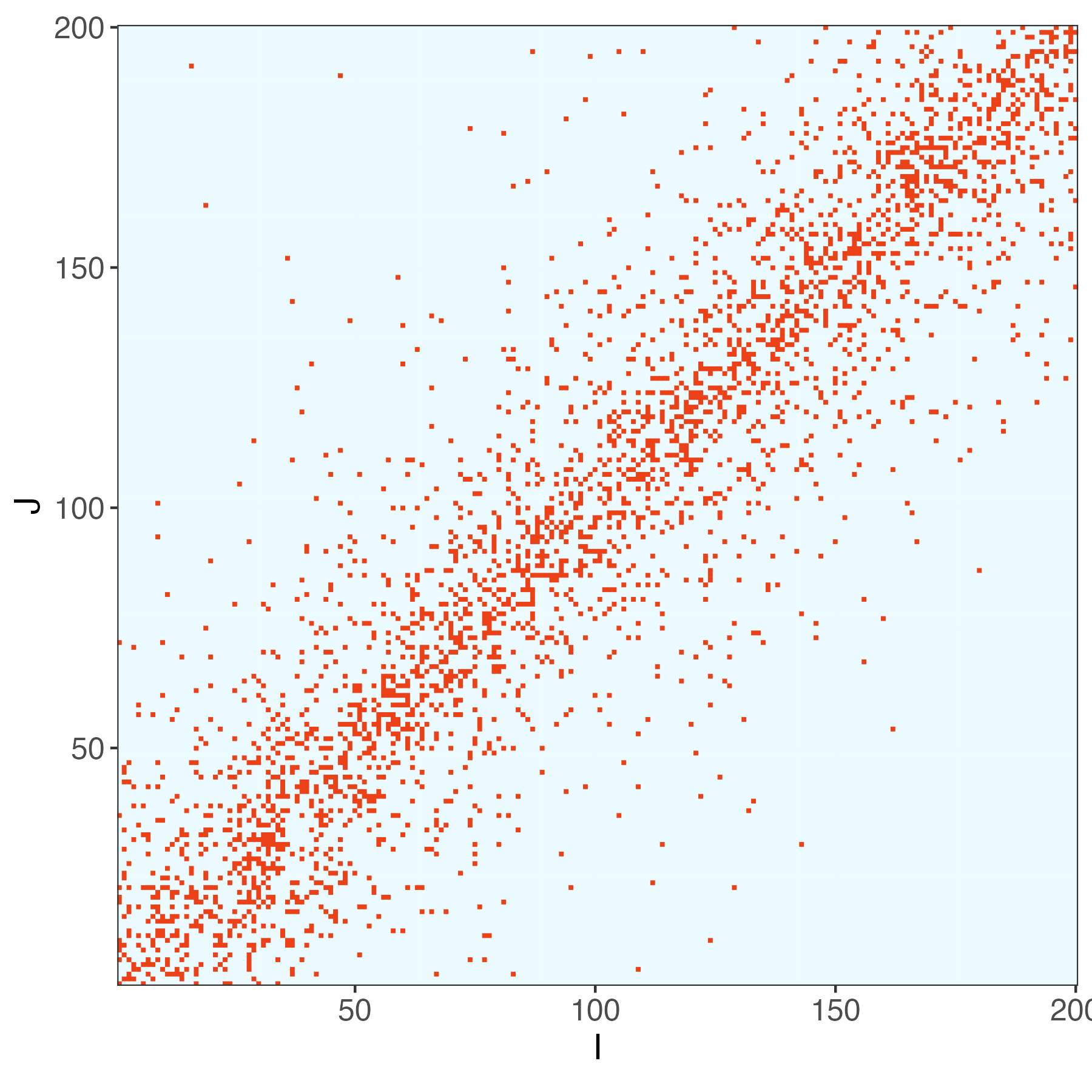
Code Demo
We simulated a SNP-histone marker association dataset x_{n} \in \{0, 1\}^{I} and y_{n} \in \reals^{J}.
\begin{align*} y_{n} &= B x_{n} + \epsilon_{n} \\ \epsilon_{n} &\sim \mathcal{N}\left(0, 0.1^2\right) \\ x_{ni} &\sim \Bern\left(\frac{1}{2}\right) \\ B_{nj} &\sim \Bern\left(0.4 \exp\left(- \frac{1}{10}\left|\frac{i}{I} - \frac{j}{J}\right|\right)\right) \\ \end{align*}
Code Demo
We can have more generous thresholds for p-values between nearby pairs. This invests the most "budget" on the promising contexts.
Code Demo
We can have more generous thresholds for p-values between nearby pairs. This invests the most "budget" on the promising contexts.
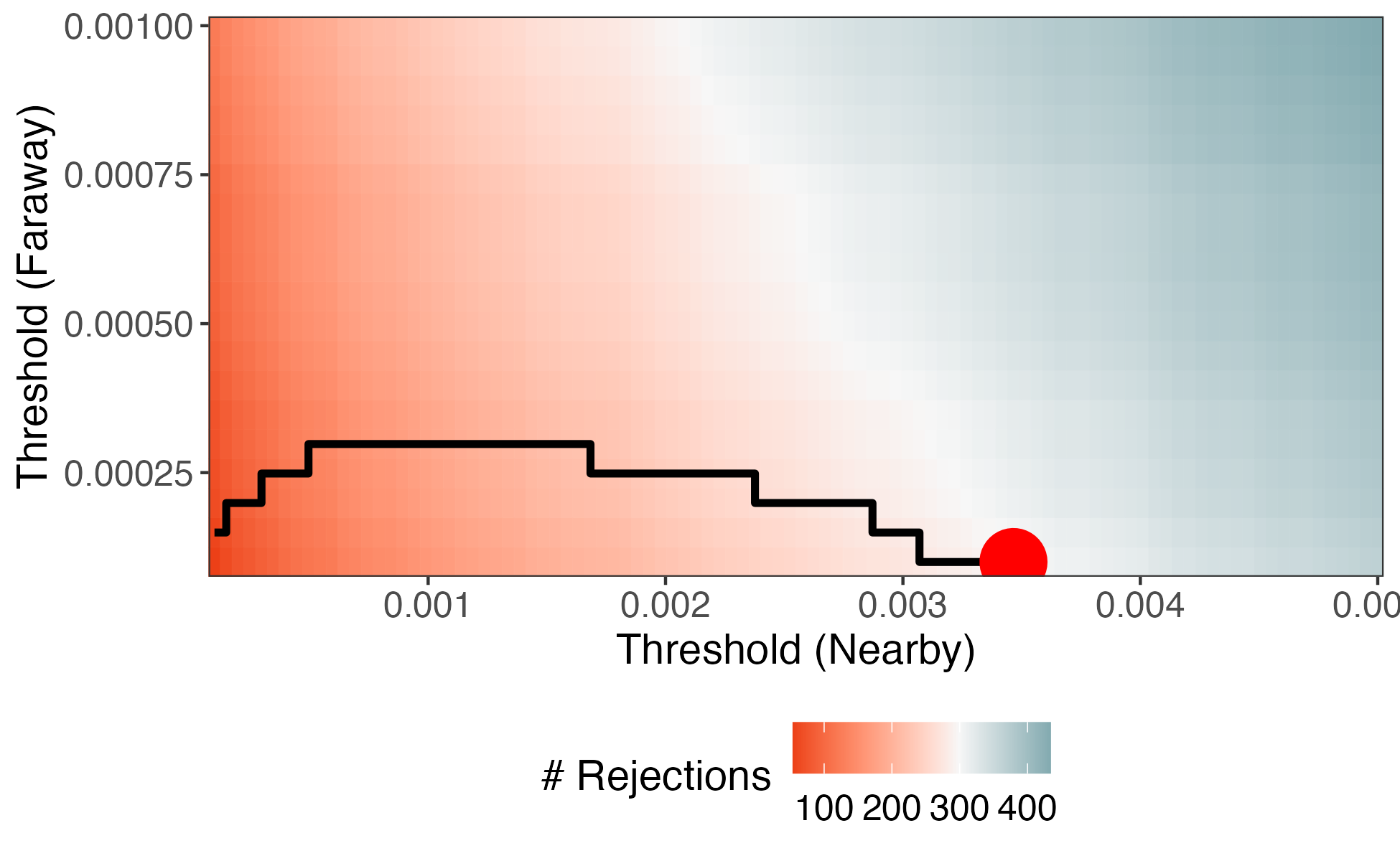
Optimization
- In practice, we would optimize \*t, rather than scanning the entire space.
- The number of rejections can be derived from the CDF of the p-value histogram, and the problem can be formulated as a convex optimization.
- We haven't discussed it, but it is important to cross-weight to ensure independence between the thresholds and p-values.
Example
- We used the
edgeRpackage to normalize these data (TMM + log transform) [7], inspired by the simulation in [8] - Notice the nonuniformity of the null p-values from the two-sample t-tests
Key Idea
We can avoid this problem if we bypass p-values altogether.
- Significance can be deduced from test statistics directly
- We do not have to use BH to ensure FDR control
This idea is highly adaptable. We'll discuss [9], but see also [10; 11].
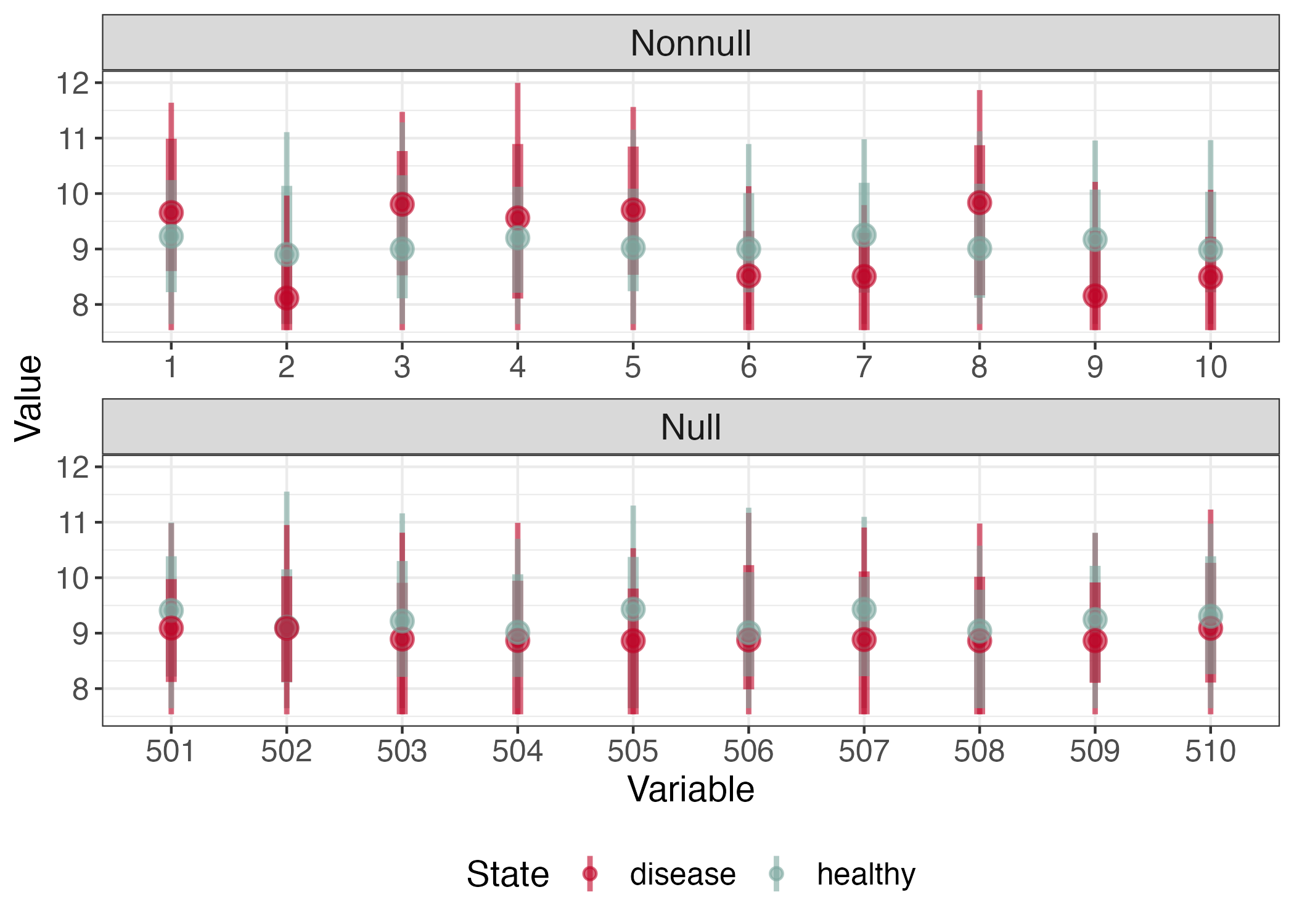
Testing \to Regression
We work with the original data \*X \in \reals^{N \times M} and \*y \in \reals^{N}. For example,
- y_{n}: Disease state for patient n
- x_{nm}: Expression level for gene m.
Consider regressing \*y = \*X \*\beta + \epsilon. The null hypothesis is that \beta_{m} = 0.
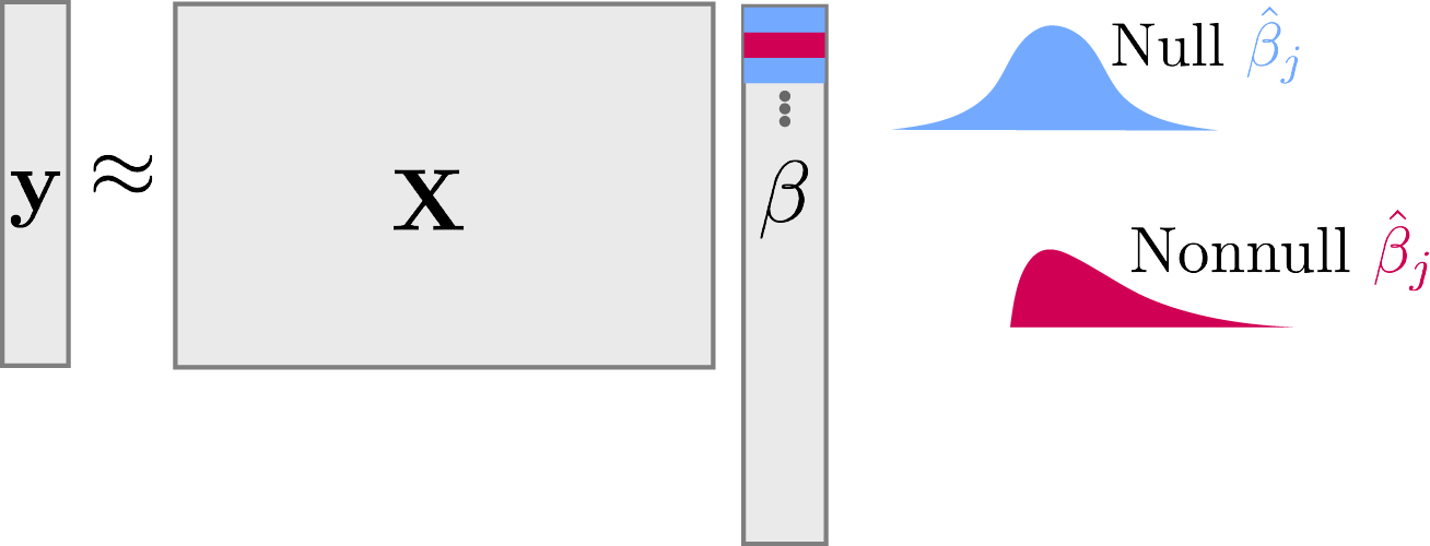
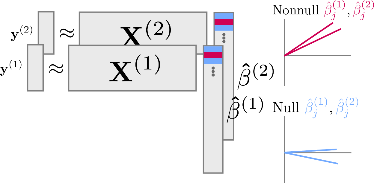
Symmetry and Mirrors
Mirror statistics measure the agreement in estimates across splits.
Example: \text{sign}\left(\hat{\beta}^{(1)}_{m}\hat{\beta}_{m}^{(2)}\right)\left[\absarg{\hat{\beta}_{m}^{(1)}} + \absarg{\hat{\beta}_{m}^{(2)}}\right]
Mirror Histogram
Let's revisit the negative binomial problem. Which hypotheses should we reject?
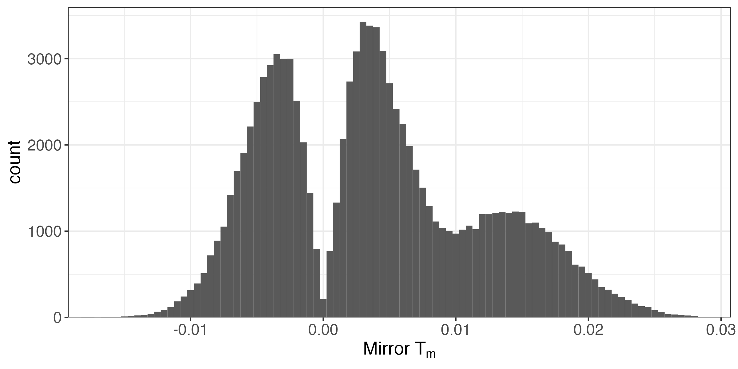
Mirror Histogram
A reasonable strategy is to reject for all T_{m} in the far right tail. How should we pick the threshold?
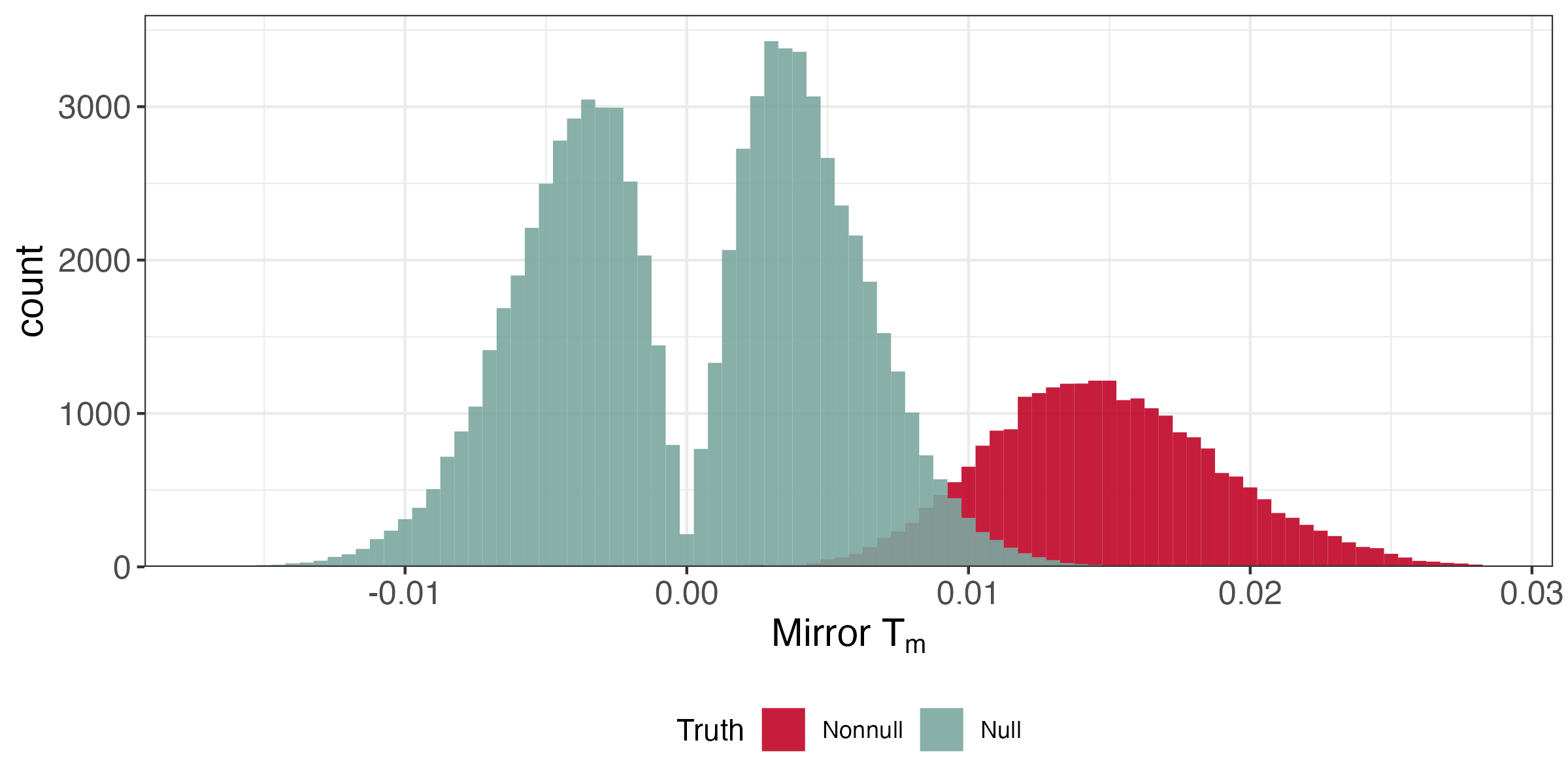
FDR Estimation
By symmetry, the size of the left tail \approx the number of nulls in the right tail,
\begin{align*} \FDR\left(t\right) &= \frac{\absarg{T_{m} < -t}}{\absarg{T_{m} > t}} \end{align*}
which suggests solving, \begin{align*} \text{maximize } &t \\ \text{subject to } &\FDR\left(t\right) \leq q \end{align*}
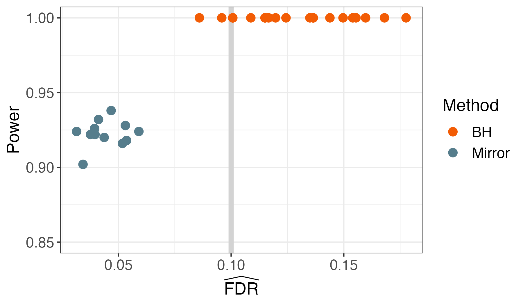
Code Demo
In our Negative Binomial example, this leads to FDR control and reasonable power. Here are the results over multiple runs.
Teaser: Microbiome Intervention Analysis
Mirror statistics support formal inference of delayed, nonlinear intervention effects in longitudinal microbiome studies [12].

Aggregation Procedure
We need a mechanism for aggregating \hat{S}_{k} across iterations.
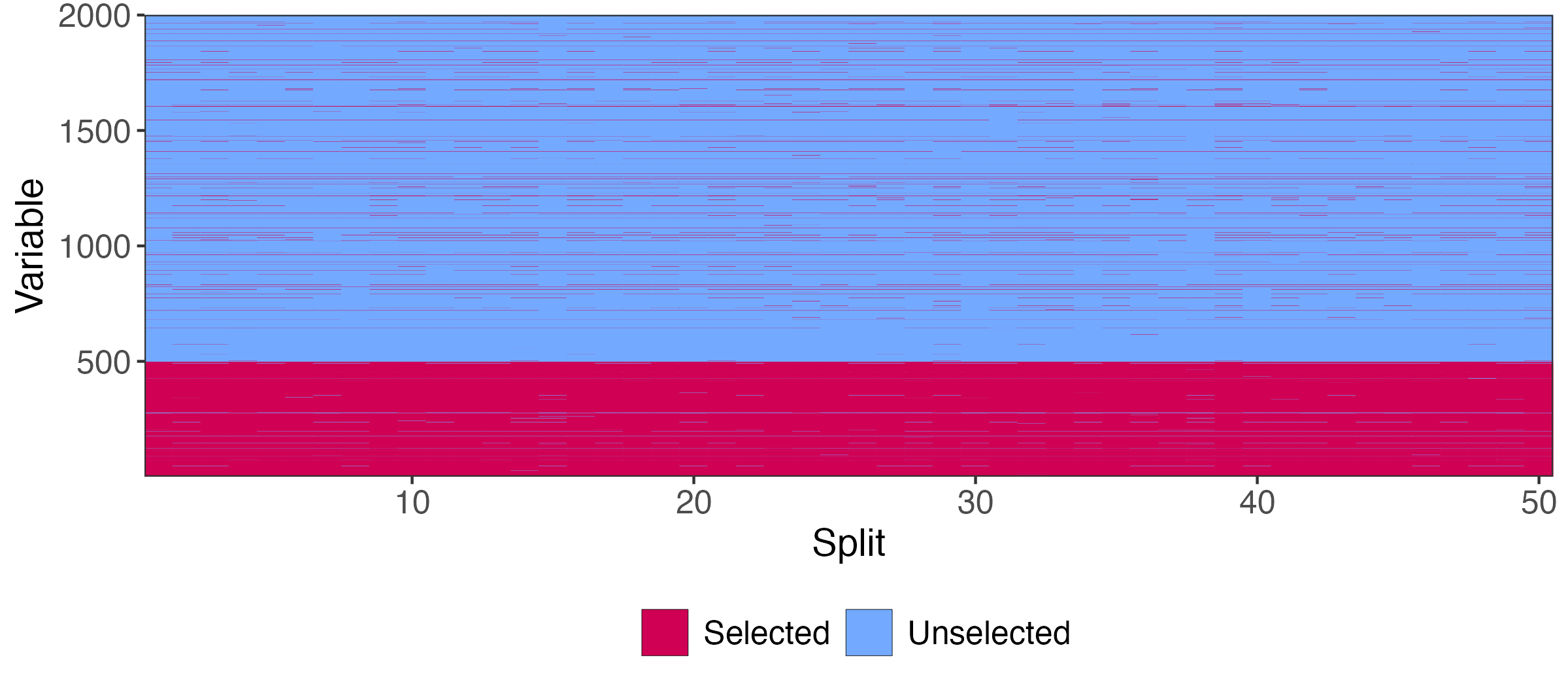
Aggregation Procedure
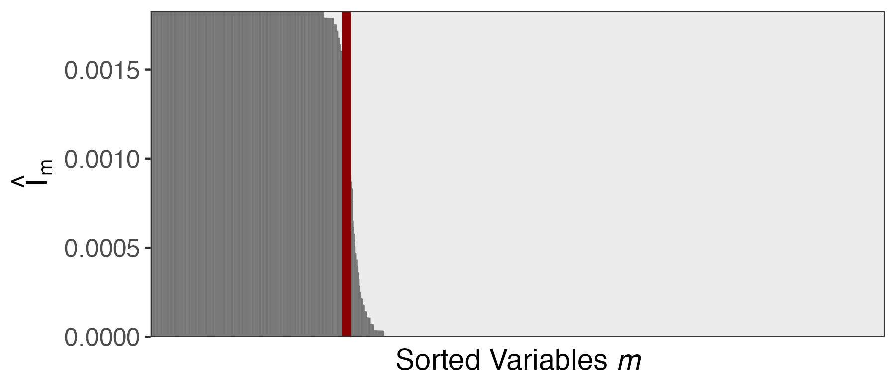
Let \hat{I}_{1}, \dots, \hat{I}_{m} store the row averages of this matrix. Larger \hat{I}_{m} means:
- The feature is selected even when \absarg{\hat{S}_{k}} is small
- The feature is selected frequently
Aggregation Procedure
Let \hat{I}_{1}, \dots, \hat{I}_{m} store the column averages of this matrix. Larger \hat{I}_{m} means:
- The feature is selected even when \absarg{\hat{S}_{k}} is small
- The feature is selected frequently
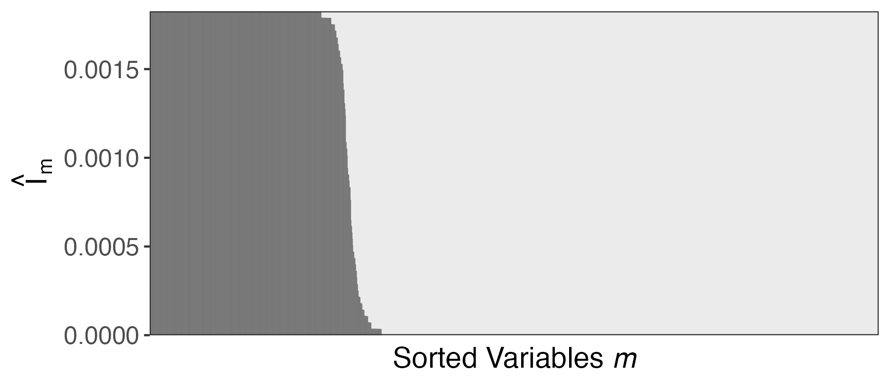
Aggregation Procedure
- For the final selection, choose features with the largest \hat{I}_{m} possible, up until the budget exceeds 1 - q.
- This is guaranteed to (asymptotically) control the FDR at level q