Linear dimensionality reduction with PCA

Code, Recording

library(tidyverse)
library(tidymodels)

1. For low-dimensional data, we could visually encode all the features in our data directly, either using properties of marks or through faceting. In high-dimensional data, this is no longer possible. However, though there are many features associated with each observation, it may still be possible to organize samples across a smaller number of meaningful, derived features. In the next week, we’ll explore a few ways of partially automating the search for relevant features.

2. An important special case for dimensionality reduction emerges when we make the following assumptions about the set of derived features,

   • Features that are linear combinations of the raw input columns.
   • Features that are orthogonal to one another.
   • Features that have high variance.

3. Why would we want features to have these properties?

   • Restricting to linear combinations allows for an analytical solution. We will relax this requirement when discussing UMAP.
   • Orthogonality means that the derived features will be uncorrelated with one another. This is a nice property, because it would be wasteful if features were redundant.
   • High variance is desirable because it means we preserve more of the essential structure of the underlying data. For example, if you look at this 2D representation of a 3D object, it’s hard to tell what it is,

   

   What is this object?

4. But when viewing an alternative reduction which has higher variance…

   

   Not so complicated now. Credit for this example goes to Professor Julie Josse, at Ecole Polytechnique.

5. Principal Components Analysis (PCA) is the optimal dimensionality reduction under these three restrictions, in the sense that it finds derived features with the highest variance. Formally, PCA finds a matrix Φ ∈ ℝ^D × K and a set of vectors z_i ∈ ℝ^K such that x_i = Φ**z_i for all i. The columns of Φ are called principal components, and they specify the structure of the derived linear features. The vector z_i is called the score of x_i with respect to these components. The top component explains the most variance, the second captures the next most, and so on. Geometrically, the columns of Φ span a plane that approximates the data. The z_i provide coordinates of points projected onto this plane.

   

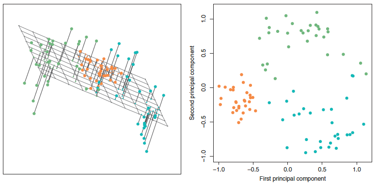
   Figure 3: PCA finds a low-dimensional linear subspace that closely approximates the high-dimensional data.

6. In R, PCA can be conveniently implemented using the tidymodels package. The dataset below contains properties of a variety of cocktails, from the Boston Bartender’s guide. The first two columns are qualitative descriptors, while the rest give numerical ingredient information.

   cocktails_df <- read_csv("https://uwmadison.box.com/shared/static/qyqof2512qsek8fpnkqqiw3p1jb77acf.csv")
   cocktails_df[, 1:6]
   
   ## # A tibble: 937 × 6
   ##    name                 category              light_rum lemon_…¹ lime_…² sweet…³
   ##    <chr>                <chr>                     <dbl>    <dbl>   <dbl>   <dbl>
   ##  1 Gauguin              Cocktail Classics          2        1       1        0  
   ##  2 Fort Lauderdale      Cocktail Classics          1.5      0       0.25     0.5
   ##  3 Cuban Cocktail No. 1 Cocktail Classics          2        0       0.5      0  
   ##  4 Cool Carlos          Cocktail Classics          0        0       0        0  
   ##  5 John Collins         Whiskies                   0        1       0        0  
   ##  6 Cherry Rum           Cocktail Classics          1.25     0       0        0  
   ##  7 Casa Blanca          Cocktail Classics          2        0       1.5      0  
   ##  8 Caribbean Champagne  Cocktail Classics          0.5      0       0        0  
   ##  9 Amber Amour          Cordials and Liqueurs      0        0.25    0        0  
   ## 10 The Joe Lewis        Whiskies                   0        0.5     0        0  
   ## # … with 927 more rows, and abbreviated variable names ¹​lemon_juice,
   ## #   ²​lime_juice, ³​sweet_vermouth
   

7. The pca_rec object below defines a tidymodels recipe for performing PCA. Computation of the lower-dimensional representation is deferred until prep() is called. This delineation between workflow definition and execution helps clarify the overall workflow, and it is typical of the tidymodels package.

   pca_rec <- recipe(~., data = cocktails_df) %>%
     update_role(name, category, new_role = "id") %>%
     step_normalize(all_predictors()) %>%
     step_pca(all_predictors())
   
   pca_prep <- prep(pca_rec)
   

8. We can tidy each element of the workflow object. Since PCA was the second step in the workflow, the PCA components can be obtained by calling tidy with the argument “2.” The scores of each sample with respect to these components can be extracted using juice. The amount of variance explained by each dimension is also given by tidy, but with the argument type = "variance".

   tidy(pca_prep, 2)
   
   ## # A tibble: 1,600 × 4
   ##    terms             value component id       
   ##    <chr>             <dbl> <chr>     <chr>    
   ##  1 light_rum        0.163  PC1       pca_tMJA6
   ##  2 lemon_juice     -0.0140 PC1       pca_tMJA6
   ##  3 lime_juice       0.224  PC1       pca_tMJA6
   ##  4 sweet_vermouth  -0.0661 PC1       pca_tMJA6
   ##  5 orange_juice     0.0308 PC1       pca_tMJA6
   ##  6 powdered_sugar  -0.476  PC1       pca_tMJA6
   ##  7 dark_rum         0.124  PC1       pca_tMJA6
   ##  8 cranberry_juice  0.0954 PC1       pca_tMJA6
   ##  9 pineapple_juice  0.119  PC1       pca_tMJA6
   ## 10 bourbon_whiskey  0.0963 PC1       pca_tMJA6
   ## # … with 1,590 more rows
   
   juice(pca_prep)
   
   ## # A tibble: 937 × 7
   ##    name                 category              PC1     PC2     PC3     PC4    PC5
   ##    <fct>                <fct>               <dbl>   <dbl>   <dbl>   <dbl>  <dbl>
   ##  1 Gauguin              Cocktail Classics   1.38  -1.15    1.34   -1.12    1.52 
   ##  2 Fort Lauderdale      Cocktail Classics   0.684  0.548   0.0308 -0.370   1.41 
   ##  3 Cuban Cocktail No. 1 Cocktail Classics   0.285 -0.967   0.454  -0.931   2.02 
   ##  4 Cool Carlos          Cocktail Classics   2.19  -0.935  -1.21    2.47    1.80 
   ##  5 John Collins         Whiskies            1.28  -1.07    0.403  -1.09   -2.21 
   ##  6 Cherry Rum           Cocktail Classics  -0.757 -0.460   0.909   0.0154 -0.748
   ##  7 Casa Blanca          Cocktail Classics   1.53  -0.392   3.29   -3.39    3.87 
   ##  8 Caribbean Champagne  Cocktail Classics   0.324  0.137  -0.134  -0.147   0.303
   ##  9 Amber Amour          Cordials and Liqu…  1.31  -0.234  -1.55    0.839  -1.19 
   ## 10 The Joe Lewis        Whiskies            0.138 -0.0401 -0.0365 -0.100  -0.531
   ## # … with 927 more rows
   
   tidy(pca_prep, 2, type = "variance")
   
   ## # A tibble: 160 × 4
   ##    terms    value component id       
   ##    <chr>    <dbl>     <int> <chr>    
   ##  1 variance  2.00         1 pca_tMJA6
   ##  2 variance  1.71         2 pca_tMJA6
   ##  3 variance  1.50         3 pca_tMJA6
   ##  4 variance  1.48         4 pca_tMJA6
   ##  5 variance  1.37         5 pca_tMJA6
   ##  6 variance  1.32         6 pca_tMJA6
   ##  7 variance  1.30         7 pca_tMJA6
   ##  8 variance  1.20         8 pca_tMJA6
   ##  9 variance  1.19         9 pca_tMJA6
   ## 10 variance  1.18        10 pca_tMJA6
   ## # … with 150 more rows
   

9. We can interpret components by looking at the linear coefficients of the variables used to define them. From the plot below, we see that the first PC mostly captures variation related to whether the drink is made with powdered sugar or simple syrup. Drinks with high values of PC1 are usually to be made from simple syrup, those with low values of PC1 are usually made from powdered sugar. From the two largest bars in PC2, we can see that it highlights the vermouth vs. non-vermouth distinction.

10. It is often easier read the components when the bars are sorted according to their magnitude. The usual ggplot approach to reordering axes labels, using either reorder() or releveling the associated factor, will reorder all the facets in the same way. If we want to reorder each facet on its own, we can use the reorder_within function coupled with scale_*_reordered, both from the tidytext package.

11. Next, we can visualize the scores of each sample with respect to these components. The plot below shows (z_i1,z_i2). Suppose that the columns of Φ are φ₁, …, φ_K. Then, since x_i = φ₁z_i1 + φ₂z_i2, the samples have large values for variables with large component values in the coordinate directions where z_i is farther along.

12. We conclude with some characteristics of PCA, which can guide the choice between alternative dimensionality reduction methods.

    • Global structure: Since PCA is looking for high-variance overall, it tends to focus on global structure.
    • Linear: PCA can only consider linear combinations of the original features. If we expect nonlinear features to be more meaningful, then another approach should be considered.
    • Interpretable features: The PCA components exactly specify how to construct each of the derived features.
    • Fast: Compared to most dimensionality reduction methods, PCA is quite fast. Further, it is easy to implement approximate versions of PCA that scale to very large datasets.
    • Deterministic: Some embedding algorithms perform an optimization process, which means there might be some variation in the results due to randomness in the optimization. In contrast, PCA is deterministic, with the components being unique up to sign (i.e., you could reflect the components across an axis, but that is the most the results might change).