Geospatial Visualization (I)
An introduction to visualizing geospatial data
library(sf)
library(tmap)
library(terra)
library(ceramic)
library(tidyverse)
-
In the same way that time plays a central role in analysis of time series datasets, space / location is often a central element in geographic data visualization. Indeed, these two types of visualization have much longer histories than even the simple scatterplot (which only emerged in the 19th century, as the abstract analog of map).
-
There are two types of geographic data worth distinguishing between — vector and raster data. Vector data formats are used to store geometric information, like the locations of hospitals (points), trajectories of bus routes (lines), or boundaries of counties (polygons). It’s useful to think of the associated data as being spatially enriched data frames, with each row corresponding to one of these geometric features. Vector data are usually stored in .geojson, .wkt, .shp, or .topojson formats.
-
Raster data give a measurement along a spatial grid. You can think of them as spatially enriched matrices, where the metadata says where on the earth each entry of the matrix is associated with. Raster data are often stored in .tiff format.
-
There are three packages that are especially useful for working with spatial data in R.
sfandterraare designed to support manipulation of vector and raster data, respectively.tmapis a visualization package applicable to either format (or even combinations of them). -
Let’s look at some vector data. The examples below read in a road network from Brasilia (multilines), glacier boundaries in Nepal (multipolygons), and locations of hospitals in Madison (multipoints). Notice that each row is georeferenced. Try searching the lat / lon coordinates online, like this.
roads <- read_sf("https://raw.githubusercontent.com/krisrs1128/stat679_code/main/examples/week7/week7-3/brasilia_small.geojson") roads ## Simple feature collection with 13724 features and 4 fields ## Geometry type: MULTILINESTRING ## Dimension: XY ## Bounding box: xmin: -47.93837 ymin: -15.84528 xmax: -47.85206 ymax: -15.7774 ## Geodetic CRS: WGS 84 ## # A tibble: 13,724 × 5 ## id X.id addr.street addr.postcode geometry ## <chr> <chr> <chr> <chr> <MULTILINESTRING [°]> ## 1 way/5081572 way/5081572 <NA> <NA> ((-47.93837 -15.77759, -… ## 2 way/5081822 way/5081822 <NA> <NA> ((-47.87463 -15.79535, -… ## 3 way/8159668 way/8159668 <NA> <NA> ((-47.88983 -15.79309, -… ## 4 way/8504851 way/8504851 <NA> <NA> ((-47.86715 -15.7998, -4… ## 5 way/10064569 way/10064569 <NA> <NA> ((-47.85206 -15.80352, -… ## 6 way/10064602 way/10064602 <NA> <NA> ((-47.9272 -15.84528, -4… ## 7 way/10064697 way/10064697 <NA> <NA> ((-47.93122 -15.84404, -… ## 8 way/10064822 way/10064822 <NA> <NA> ((-47.93144 -15.84261, -… ## 9 way/10064844 way/10064844 <NA> <NA> ((-47.93703 -15.84485, -… ## 10 way/10064854 way/10064854 <NA> <NA> ((-47.93274 -15.84491, -… ## # … with 13,714 more rows clinics <- read_sf("https://raw.githubusercontent.com/krisrs1128/stat679_code/main/examples/week7/week7-3/clinics.geojson") clinics ## Simple feature collection with 30 features and 33 fields ## Geometry type: GEOMETRY ## Dimension: XY ## Bounding box: xmin: -89.52806 ymin: 43.00435 xmax: -89.3083 ymax: 43.12346 ## Geodetic CRS: WGS 84 ## # A tibble: 30 × 34 ## id X.id addr.…¹ addr.…² addr.…³ addr.…⁴ addr.…⁵ addr.…⁶ addr.…⁷ alt_n…⁸ ## <chr> <chr> <chr> <chr> <chr> <chr> <chr> <chr> <chr> <chr> ## 1 way/38… way/… Madison 8202 53717 WI Excels… <NA> <NA> <NA> ## 2 way/10… way/… Madison 675 53703 <NA> West W… <NA> <NA> <NA> ## 3 way/10… way/… <NA> <NA> <NA> <NA> <NA> <NA> <NA> <NA> ## 4 way/10… way/… Madison 3706 53704 WI Orin R… <NA> <NA> <NA> ## 5 way/10… way/… Madison 1500 53705 <NA> Highla… <NA> <NA> <NA> ## 6 way/10… way/… <NA> <NA> <NA> <NA> <NA> <NA> <NA> <NA> ## 7 way/13… way/… <NA> <NA> <NA> <NA> <NA> <NA> <NA> <NA> ## 8 way/15… way/… <NA> <NA> <NA> <NA> <NA> <NA> <NA> <NA> ## 9 way/20… way/… <NA> <NA> <NA> <NA> <NA> <NA> <NA> <NA> ## 10 way/22… way/… Madison 3102 <NA> WI Merite… <NA> <NA> <NA> ## # … with 20 more rows, 24 more variables: amenity <chr>, brand <chr>, ## # brand.wikidata <chr>, brand.wikipedia <chr>, building <chr>, ## # building.levels <chr>, emergency <chr>, gnis.feature_id <chr>, ## # healthcare <chr>, healthcare.counselling <chr>, ## # healthcare.speciality <chr>, internet_access <chr>, layer <chr>, ## # name <chr>, name.en <chr>, opening_hours <chr>, operator <chr>, ## # phone <chr>, roof.levels <chr>, start_date <chr>, … glaciers <- read_sf("https://raw.githubusercontent.com/krisrs1128/stat679_code/main/examples/week7/week7-3/glaciers.geojson") glaciers ## Simple feature collection with 108 features and 21 fields ## Geometry type: MULTIPOLYGON ## Dimension: XY ## Bounding box: xmin: 80.80884 ymin: 29.90459 xmax: 81.01887 ymax: 30.17747 ## Geodetic CRS: WGS 84 ## # A tibble: 108 × 22 ## ID GLIMS_ID Basin Sub_B…¹ Images Longi…² Latit…³ Class Elv_min Elv_m…⁴ ## <dbl> <chr> <chr> <chr> <chr> <dbl> <dbl> <chr> <int> <int> ## 1 3 G080926E301… Maha… Mahaka… l5144… 80.9 30.2 53012 4426 4895 ## 2 5 G080955E301… Maha… Mahaka… l5144… 81.0 30.2 64022 4782 5185 ## 3 8 G080932E301… Maha… Mahaka… l5144… 80.9 30.2 67023 4968 5060 ## 4 23 G081016E300… Maha… Mahaka… l5144… 81.0 30.1 63022 4965 5012 ## 5 24 G080856E300… Maha… Mahaka… l5144… 80.9 30.1 63022 4611 4814 ## 6 26 G080939E300… Maha… Mahaka… l5144… 80.9 30.0 67023 5355 5522 ## 7 27 G080861E300… Maha… Mahaka… l5144… 80.9 30.0 67023 4907 5010 ## 8 28 G080951E300… Maha… Mahaka… l5144… 81.0 30.0 53012 3695 4777 ## 9 29 G080879E300… Maha… Mahaka… l5144… 80.9 30.0 65052 4979 5127 ## 10 30 G080876E300… Maha… Mahaka… l5144… 80.9 30.0 67023 5183 5296 ## # … with 98 more rows, 12 more variables: Elv_max <int>, Slope_min <int>, ## # Slope_mean <int>, Slope_max <int>, Aspect <int>, Area_SqKm <dbl>, ## # Thickness <dbl>, Reserve <dbl>, Year <int>, Shape_area <dbl>, ## # Shape_len <dbl>, geometry <MULTIPOLYGON [°]>, and abbreviated variable ## # names ¹Sub_Basin, ²Longitude, ³Latitude, ⁴Elv_mean -
We will use
tmapto visualize each of these datasets. The logic of the package mirrors that ofggplot2, we usetmap_shapeto tell the package our source data, and then we can add on layers that add visual marks based on it. For example, to draw the road network, we use add on atmap_linelayer. For the glaciers and hospitals, we can use the analogous fill and point layers.tm_shape(roads) + tm_lines()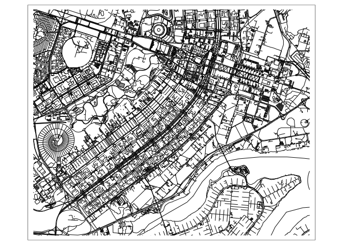
tm_shape(clinics) +
  tm_dots(size = 1, col = "red")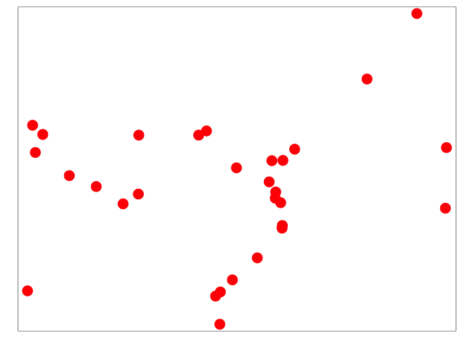
tm_shape(glaciers) +
  tm_polygons()
-
Remember that each element of a vector dataset can be thought of as a row of a data.frame (just with added georeferencing information). This means that it is often possible to encode features of each element using properties of the marks used to represent them. For example, we’ve shaded in each of the glaciers by their thickness, which shows that the larger and more central ones tend to be thicker. These kinds of fill-encoded polygon visualizations are sometimes called choropleths.
tm_shape(glaciers) +
  tm_borders() +
  tm_fill(col = "Thickness", palette = "Blues", legend.hist = TRUE) +
  tm_layout(legend.outside = TRUE)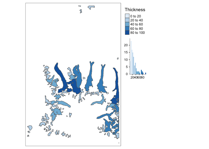
-
What about raster data? We can again use
tmap, but we have to use different types of layers. For example, the data read in below come from the Sentinel 2 satellite, an open (and continually updated) collection of satellite images maintained by the European Space Agency. They give imagery associated with one small subset of the glaciers labels. To visualize just one image channel from this data, we can usetmap_raster.im <- rast("https://uwmadison.box.com/shared/static/lpmujy5odtt3otpq1bluiv16fkg0o4t2.tif") %>% stretch() # only the first layer tm_shape(subset(im, 1)) + tm_raster()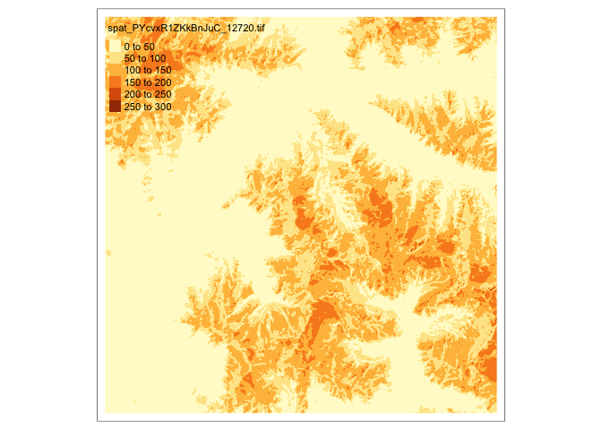
-
Many raster datasets have more than just one channel (our Sentinel dataset has 13). We can plot combinations of them using
tmap_rgb. For example, channels 2 - 4 correspond to the usual RGB channels that appear in ordinary camera images.tm_shape(im) + tm_rgb()
-
We can overlay vector data over a raster basemap by combining layers. We are retrieving the basemap using the
cc_locationfunction inceramic.# you can get your own at https://account.mapbox.com/access-tokens/ Sys.setenv(MAPBOX_API_KEY="pk.eyJ1Ijoia3Jpc3JzMTEyOCIsImEiOiJjbDYzdjJzczQya3JzM2Jtb2E0NWU1a3B3In0.Mk4-pmKi_klg3EKfTw-JbQ") basemap <- cc_location(loc= c(-89.401230, 43.073051), buffer = 15e3) ## Preparing to download: 16 tiles at zoom = 12 from ## https://api.mapbox.com/v4/mapbox.satellite/ tm_shape(basemap) + tm_rgb() + tm_shape(clinics) + tm_dots(col = "red", size = 1)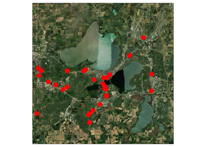
-
In all the discussion above, we’ve worked with the original spatial data that were given to us. In practice, we will often want to manipulate these data before making a final visualization — for example, we may want to crop to a specific region of interest or unify sources from a few neighboring regions. These types of operations are the bread and butter of
sfandterra. For example, if we want to crop the glacier labels down to the region contained by the satellite image, we can usesf’sst_cropcommand. -
We can also zoom into the raster data using
terra’s crop function. We crop both datasets again to get a high-resolution view of this region.e <- ext(80.7, 81, 29.9, 30) im_crop <- crop(im, e) glaciers_crop <- st_crop(glaciers, e) tm_shape(im_crop) + tm_rgb() + tm_shape(glaciers_crop) + tm_polygons(col = "Thickness", palette = "Blues", legend.hist = TRUE, alpha = 0.5) + tm_layout(legend.outside = TRUE)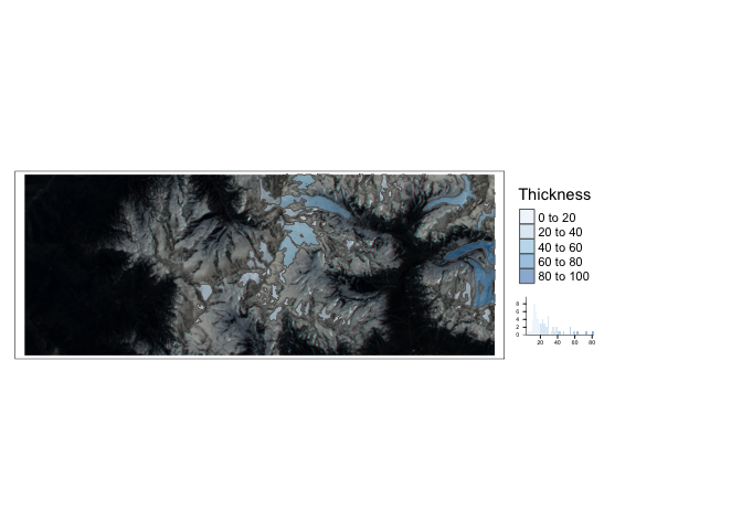
-
tmapprovides many functions for customizing the appearance of our maps. For example, there are layers for adding specific cartographic elements, like bar scales (tmap_scale_bar) and compasses (tmap_compass). Moreover, the themes and layout of the existing layers can be adapted using thetmap_layoutfunction – this is how we customized the fill colors and legend properties above.