Introduction to Topic Modeling

2022-06-02 00:00

Quantitative descriptions of document topics

library(tidyverse)
library(tidytext)
library(topicmodels)
library(gutenbergr) # devtools::install_github("ropensci/gutenbergr")

Topic modeling is a type of dimensionality reduction method that is especially useful for high-dimensional count matrices. For example, it can be applied to,
- Text data analysis, where each row is a document and each column is a word. The i**j entry contains the count of word j word in the document i.
- Gene expression analysis, where each row is a biological sample and each column is a gene. The i**j entry measures the amount of gene j expressed in sample i.
This week, we’ll specifically focus on the application to text data, since otherwise, we’ve covered relatively few visualization techniques that can be applied to this (very common) type of data. For the rest of these lectures, we’ll refer to samples as documents and features as words, even though these methods can be used more generally.
These models are useful to know about because they provide a compromise between clustering and PCA.
- In clustering, each document would have to be assigned to a single topic. In contrast, topic models allow each document to partially belong to several topics simultaneously. In this sense, they are more suitable when data do not belong to distinct, clearly-defined clusters.
- PCA is also appropriate when the data vary continuously, but it does not provide any notion of clusters. In contrast, topic models estimate K topics, which are analogous to a cluster centroids (though documents are typically a mix of several centroids).
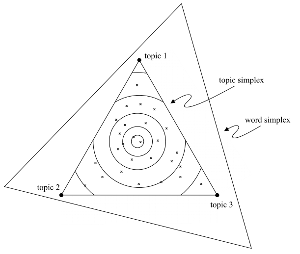
Without going into mathematical detail, topic models perform dimensionality reduction by supposing, (i) each document is a mixture of topics and (ii) each topic is a mixture of words. For (i), consider modeling a collection of newspaper articles. A set of articles might belong primarily to the “politics” topic, and others to the “business” topic. Articles that describe a monetary policy in the federal reserve might belong partially to both the “politics” and the “business” topic. For (ii), consider the difference in words that would appear in politics and business articles. Articles about politics might frequently include words like “congress” and “law,” but only rarely words like “stock” and “trade.”
A document is a mixture of topics, with more words coming from the topics that it is close to. More precisely, a document that is very close to a particular topic has a word distribution just like that topic. A document that is intermediate between two topics has a word distribution that mixes between both topics.
Let’s see how to fit a topic model in R. We will use LDA as implemented in the topicmodels package, which expects input to be structured as a DocumentTermMatrix, a special type of matrix that stores the counts of words (columns) across documents (rows). In practice, most of the effort required to fit a topic model goes into transforming the raw data into a suitable DocumentTermMatrix.

To illustrate this process, let’s consider the “Great Library Heist” example from the reading. We imagine that a thief has taken four books — Great Expectations, Twenty Thousand Leagues Under The Sea, War of the Worlds, and Pride & Prejudice — and torn all the chapters out. We are left with pieces of isolated pieces of text and have to determine from which book they are from. The block below downloads all the books into an R object.

titles <- c("Twenty Thousand Leagues under the Sea",
        "The War of the Worlds",
        "Pride and Prejudice", 
        "Great Expectations")
books <- gutenberg_works(title %in% titles) %>%
  gutenberg_download(meta_fields = "title")
books

## # A tibble: 53,724 × 3
##    gutenberg_id text                    title                
##           <int> <chr>                   <chr>                
##  1           36 "cover "                The War of the Worlds
##  2           36 ""                      The War of the Worlds
##  3           36 ""                      The War of the Worlds
##  4           36 ""                      The War of the Worlds
##  5           36 ""                      The War of the Worlds
##  6           36 "The War of the Worlds" The War of the Worlds
##  7           36 ""                      The War of the Worlds
##  8           36 "by H. G. Wells"        The War of the Worlds
##  9           36 ""                      The War of the Worlds
## 10           36 ""                      The War of the Worlds
## # … with 53,714 more rows

Since we imagine that the word distributions are not equal across the books, topic modeling is a reasonable approach for discovering the books associated with each chapter. Let’s start by simulating the process of tearing the chapters out. We split the raw texts anytime the word “Chapter” appears. We will keep track of the book names for each chapter, but this information is not passed into the topic modeling algorithm.
```
by_chapter <- books %>%
  group_by(title) %>%
  mutate(
    chapter = cumsum(str_detect(text, regex("chapter", ignore_case = TRUE)))
  ) %>%
  group_by(title, chapter) %>%
  mutate(n = n()) %>%
  filter(n > 5) %>%
  ungroup() %>%
  unite(document, title, chapter)
```
As it is, the text data are long character strings, giving actual text from the novels. To fit LDA, we only need counts of each word within each chapter – the algorithm throws away information related to word order. To derive word counts, we first split the raw text into separate words using the unest_tokens function in the tidytext package. Then, we can count the number of times each word appeared in each document using count, a shortcut for the usual group_by and summarize(n = n()) pattern.
```
word_counts <- by_chapter %>%
  unnest_tokens(word, text) %>%
  anti_join(stop_words) %>%
  count(document, word)
```
These words counts are still not in a format compatible with conversion to a DocumentTermMatrix. The issue is that the DocumentTermMatrix expects words to be arranged along columns, but currently they are stored across rows. The line below converts the original “long” word counts into a “wide” DocumentTermMatrix in one step. Across these 4 books, we have 65 chapters and a vocabulary of size 18325.
```
chapters_dtm <- word_counts %>%
  cast_dtm(document, word, n)
```
Once the data are in this format, we can use the LDA function to fit a topic model. We choose K = 4 topics because we expect that each topic will match a book. Different hyperparameters can be set using the control argument. There are two types of outputs produced by the LDA model: the topic word distributions (for each topic, which words are common?) and the document-topic memberships (from which topics does a document come from?). For visualization, it will be easiest to extract these parameters using the tidy function, specifying whether we want the topics (beta) or memberships (gamma).
```
chapters_lda <- LDA(chapters_dtm, k = 4, control = list(seed = 1234))
chapters_lda

## A LDA_VEM topic model with 4 topics.

topics <- tidy(chapters_lda, matrix = "beta")
memberships <- tidy(chapters_lda, matrix = "gamma")
```

This tidy approach is preferable to extracting the parameters directly from the fitted model (e.g., using chapters_lda@gamma) because it ensures the output is a tidy data.frame, rather than a matrix. Tidy data.frames are easier to visualize using ggplot2.

# highest weight words per topic
topics %>%
  arrange(topic, -beta)

## # A tibble: 74,976 × 3
##    topic term          beta
##    <int> <chr>        <dbl>
##  1     1 captain    0.0153 
##  2     1 _nautilus_ 0.0126 
##  3     1 sea        0.00907
##  4     1 nemo       0.00863
##  5     1 ned        0.00789
##  6     1 conseil    0.00676
##  7     1 water      0.00599
##  8     1 land       0.00598
##  9     1 sir        0.00485
## 10     1 day        0.00365
## # … with 74,966 more rows

# topic memberships per document
memberships %>%
  arrange(document, topic)

## # A tibble: 780 × 3
##    document               topic     gamma
##    <chr>                  <int>     <dbl>
##  1 Great Expectations_0       1 0.00282  
##  2 Great Expectations_0       2 0.461    
##  3 Great Expectations_0       3 0.00282  
##  4 Great Expectations_0       4 0.533    
##  5 Great Expectations_100     1 0.000424 
##  6 Great Expectations_100     2 0.000424 
##  7 Great Expectations_100     3 0.999    
##  8 Great Expectations_100     4 0.000424 
##  9 Great Expectations_101     1 0.0000140
## 10 Great Expectations_101     2 0.0000140
## # … with 770 more rows

save(topics, memberships, file = "12-1.rda")

Statistical Data Visualization