Nonlinear dimensionality reduction with UMAP

Code, Recording

1. Nonlinear dimension reduction methods can give a more faithful representation than PCA when the data don’t lie on a low-dimensional linear subspace. For example, suppose the data were shaped like this. There is no one-dimensional line through these data that separate the groups well. We will need an alternative approach to reducing dimensionality if we want to preserve nonlinear structure.

   library(tidyverse)
   library(embed)
   theme_set(theme_minimal())
   
   moons <- read_csv("https://uwmadison.box.com/shared/static/kdt9qqvonhcz2ssb599p1nqganrg1w6k.csv")
   ggplot(moons, aes(X, Y, col = Class)) +
     geom_point() +
     scale_color_brewer(palette = "Set2")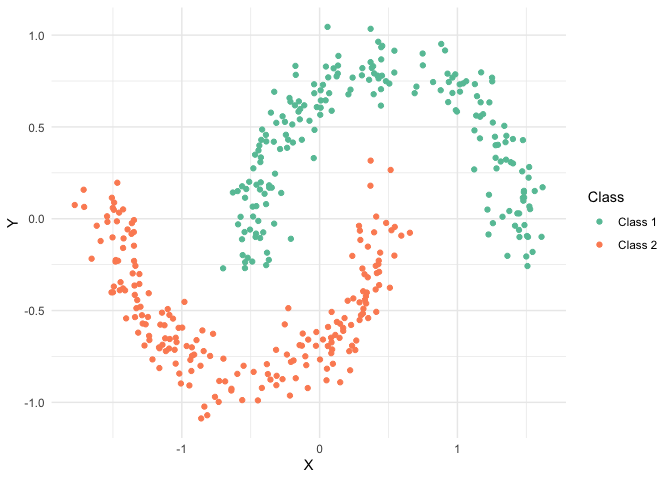
   

   

2. From a high-level, the intuition behind UMAP is to (a) build a graph joining nearby neighbors in the original high-dimensional space, and then (b) layout the graph in a lower-dimensional space. For example, consider the 2-dimensional sine wave below. If we build a graph, we can try to layout the resulting nodes and edges on a 1-dimensional line in a way that approximately preserves the ordering.

   

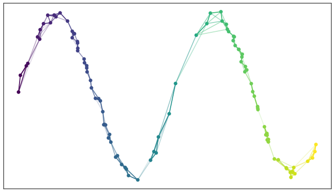
   UMAP (and many other nonlinear methods) begins by constructing a graph in the high-dimensional space, whose layout in the lower dimensional space will ideally preserve the essential relationships between samples.

3. A natural way to build a graph is to join each node to its K closest neighbors. The choice of K will influence the final reduction, and it is treated as a hyperparameter of UMAP. Larger values of K prioritize preservation of global structure, while smaller K will better reflect local differences. This property is not obvious a priori, but is suggested by the simulations described in the reading.

   

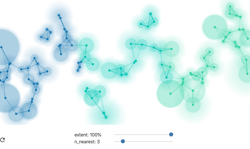
   When using fewer nearest neighbors, the final dimensionality reduction will place more emphasis on effectively preserving the relationships between points in local neighborhoods.

4. One detail in the graph construction: In UMAP, the edges are assigned weights depending on the distance they span, normalized by the distance to the closest neighbor. Neighbors that are close, relative to the nearest neighbors, are assigned higher weights than those that are far away, and points that are linked by high weight edges are pulled together with larger force in the final graph layout. This is what the authors mean by using a ``fuzzy’’ nearest neighbor graph. The fuzziness allows the algorithm to distinguish neighbors that are very close from those that are far, even though they all lie within a K-nearest-neighborhood.

   

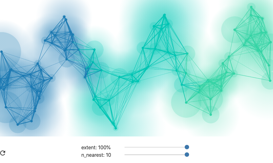
   When using larger neighborhoods, UMAP will place more emphasis on preserving global structure, sometimes at the cost of local relationships between points.

5. Once the graph is constructed, there is the question of how the graph layout should proceed. UMAP uses a variant of force-directed layout, and the global strength of the springs is another hyperparameter. Lower tension on the springs allow the points to spread out more loosely, higher tension forces points closer together. This is a second hyperparameter of UMAP.

   

6. In R, we can implement this using almost the same code as we used for PCA. The step_umap command is available through the embed package.

   theme_set(theme_bw())
   cocktails_df <- read_csv("https://uwmadison.box.com/shared/static/qyqof2512qsek8fpnkqqiw3p1jb77acf.csv")
   umap_rec <- recipe(~., data = cocktails_df) %>%
     update_role(name, category, new_role = "id") %>%
     step_normalize(all_predictors()) %>%
     step_umap(all_predictors(), neighbors = 20, min_dist = 0.1)
   umap_prep <- prep(umap_rec)
   ggplot(juice(umap_prep), aes(UMAP1, UMAP2)) +
     geom_point(aes(color = category), alpha = 0.7, size = 0.8) +
     geom_text(aes(label = name), check_overlap = TRUE, size = 3, hjust = "inward")
   

   

7. We can summarize the properties of UMAP,

   • Global or local structure: The number of nearest neighbors K used during graph construction can be used modulate the emphasis of global vs. local structure.
   • Nonlinear: UMAP can reflect nonlinear structure in high-dimensions.
   • No interpretable features: UMAP only returns the map between points, and there is no analog of components to describe how the original features were used to construct the map.
   • Slower: While UMAP is much faster than comparable nonlinear dimensionality reduction algorithms, it is still slower than linear approaches.
   • Nondeterministic: The output from UMAP can change from run to run, due to randomness in the graph layout step. If exact reproducibility is required, a random seed should be set.