Tree Representations

2022-06-01 00:00

An important special case of graph data visualization

library(tidygraph)
library(ggraph)
library(patchwork)
theme_set(theme_bw())

Formally, trees are a special type of graph which have no cycles (paths starting at one node that can return without retracing any steps). Informally, they can be thought of as hierarchies descending from a “root” node. These notes review some techniques for visualizing tree structured data.

One approach is to encode each node’s depth in the tree by using vertical or radial position. To illustrate, we’ll work with the following dataset, which shows the directory structure of an open source software package called flare.

G_flare <- tbl_graph(flare$vertices, flare$edges)
G_flare

## # A tbl_graph: 252 nodes and 251 edges
## #
## # A rooted tree
## #
## # Node Data: 252 × 3 (active)
##   name                                          size shortName            
##   <chr>                                        <dbl> <chr>                
## 1 flare.analytics.cluster.AgglomerativeCluster  3938 AgglomerativeCluster 
## 2 flare.analytics.cluster.CommunityStructure    3812 CommunityStructure   
## 3 flare.analytics.cluster.HierarchicalCluster   6714 HierarchicalCluster  
## 4 flare.analytics.cluster.MergeEdge              743 MergeEdge            
## 5 flare.analytics.graph.BetweennessCentrality   3534 BetweennessCentrality
## 6 flare.analytics.graph.LinkDistance            5731 LinkDistance         
## # … with 246 more rows
## #
## # Edge Data: 251 × 2
##    from    to
##   <int> <int>
## 1   221     1
## 2   221     2
## 3   221     3
## # … with 248 more rows

In ggraph, this kind of visualization is constructed using the same type of node-link geoms as before. We can organize nodes by depth (distance from the root) by specifying that the layout be tree.

p1 <- ggraph(G_flare, "tree") +
  geom_edge_link() +
  geom_node_label(aes(label = shortName), size = 3)

p2 <- ggraph(G_flare, "tree", circular = TRUE) +
  geom_edge_link() +
  geom_node_label(aes(label = shortName), size = 3)

p1 | p2

How can we begin to make similar figures with D3? We need to be able to find coordinates for both nodes and links across the tree. Once we have these coordinates, we can append corresponding circle and path SVG elements. There are three main steps before we can reach this point,
- Convert the flat array containing the list of edges into a stratified JS object that can be input to the next steps. This is done with d3.stratify(). The resulting stratified object also includes many useful helper methods, like calculation of all the descendants of a node or identification of which nodes are leaves.
- Given the stratified object, define the tree layout. It also associates each node with an x and y pixel coordinate. This can be done with d3.tree().
- If we want smooth edges between parent and child nodes, we need a path generator. This generator is used to define the d attributes of the SVG paths for each link. This can be done using d3.linkVertical() (for vertical trees) or d3.linkHorizontal() (for trees on their sides).
For example, to draw a tree for the flare dataset, we start with a flat array of edges. Note that the first element is the root – the node with no parents,
```
[
  {from: null, to: "flare"},
  {from: "flare", to: "flare.analytics"},
  {from: "flare", to: "flare.vis"},
  {from: "flare.vis", to: "flare.vis.operator"},
  ...
]
```
We define a function that stratifies this flat edge array using the following syntax. The id and parentId methods parse the parent-child relationship structure from each array element.
```
let stratifier = d3.stratify()
  .id(d => d.to)
  .parentId(d => d.from)
```
Calling the stratifier on the original edgelist creates the nested data structure shown below. Notice that it has automatically calculated many useful properties, like the node’s depth in the tree and the data from its parent.
```
stratifier(edge_array)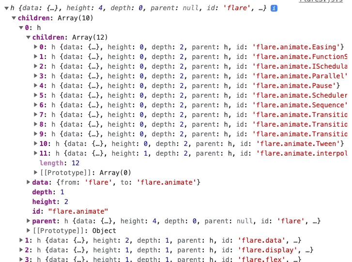
```
The really wonderful thing about the stratified object is that it includes many helper methods which allow us to avoid manually implementing common tree operations. For example, the call below will return the 22 nodes descending from the first child of the root (since the children are sorted alphabetically, this node is flare.animate).
```
stratified = stratifier(data["edges"])
stratified.children[0].descendants()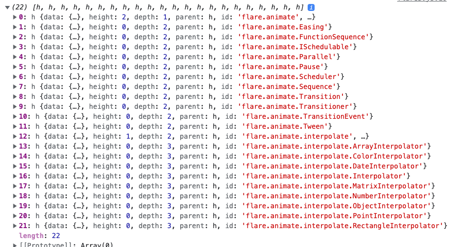
```
Next, we call d3.tree() on the stratified object. This is what calculates the pixel coordinates of each node along the tree. The .size() method below specifies the maximum x and y coordinates of the final layout. In the screenshot below, you can see that the above stratified object now includes .x and .y attributes for each node.
```
tree_gen = d3.tree().size([600, 350])
let tree = tree_gen(stratified)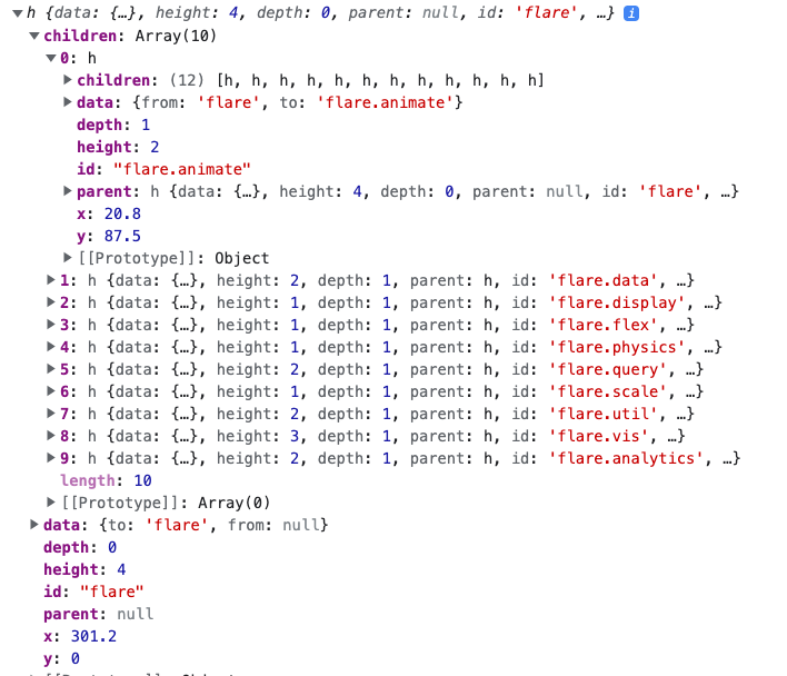
```
In order to bind data using the general update pattern, we’re going to need convert these data back into arrays. Fortunately, there are two methods, .links() and .descendants(), which let us retrieve edge and node arrays from this stratified object. Unlike the edge data we had initially read in, this modified edge array also includes x and y coordinate information, thanks to the previous call to d3.tree(). For example, this will bind circles associated with each node in the tree.
```
d3.select("#tree")
  .selectAll("circle")
  .data(tree.descendants()).enter()
  .append("circle")
  .attrs({
    cx: d => d.x,
    cy: d => d.y,
    ...
  })
```
If we want curved edges, we can use a special path generator, called d3.linkVertical(), designed to draw tree links. The resulting tree is shown below. We could always have used a d3.line() generator to draw the path, but those edges would be straight paths from one node to the next.
```
let link_gen = d3.linkVertical()
  .x(d => d.x)
  .y(d => d.y);

d3.select("#tree")
  .selectAll("path")
  .data(tree.links()).enter()
  .append("path")
  .attrs({
    d: link_gen,
    ...
  })
```
This seems like a lot of work just to create a simple tree. As usual with D3, the real value becomes apparent when we want to build in some interactivity. Here is an example of the same tree but which highlights all ancestor and descendant nodes whenever the mouse is moved near one node. We’ll over the details during a class demo – if you are curious, you can read the full implementation here.
We’ve spent quite a bit of time going over how to display trees using node-link diagrams. There is one other very common tree representation that is worth knowing: treemaps. The idea is to encode parent-child relationships using enclosure (i.e., the containment of some visual marks within others).
In the visualization below, each node is allocated an area, and all its children are drawn within that area (and so on, recursively, down to the leaves). The first two lines of code are the most important. The first says that we want to use a treemap layout, and the size of each node should reflect the size column in the nodes component of G_flare. The second line specifies visual encodings to add to each treemap tile – the color will reflect how deep we are into the tree.
```
    ggraph(G_flare, "treemap", weight = size) +
      geom_node_tile(aes(fill = depth)) +
      scale_fill_distiller(direction = 1) +
      coord_fixed()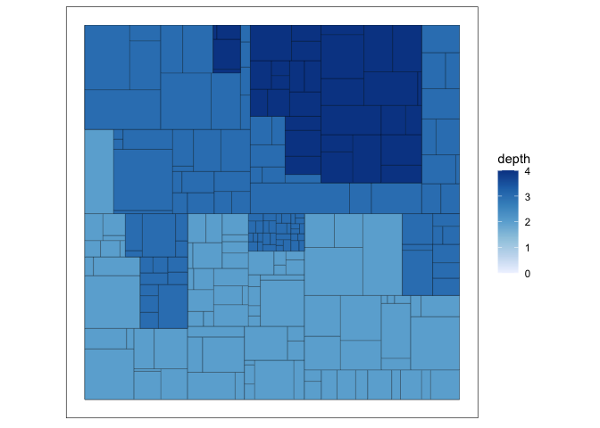
```
This is a particularly useful visualization when it’s important to visualize a continuous attribute associated with each node. In the above example, the size of each tile was was determined by the size variable. For example, a large node might correspond to a large part of a budget or a large directory in a filesystem. The main difficulty with using enclosure is that it becomes more difficult to trace the parent-child structure of the tree. Connections between nodes immediately stand out in the node-link diagram, but they require deliberate inspection when using treemaps.
In D3, the analogous code is generated using the d3.treemap() function. Though the layout is quite different, the way in which it is applied to a stratified data object is very similar to the use of d3.tree(). The source code can be read here – note that d3.stratify() was not needed here, because the input data are already a stratified object (not just an array of edges).
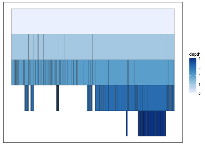
An intermediate between the node-link and the treemap approach is to use an icicle plot. In this approach, the distance from the root is still encoded using position, like in a node-link diagram. A continuous value can be associated with each descendant node and encoded encoded using the length of the associated rectangle. In ggraph, we can create this by specifying a “partition” layout.

ggraph(G_flare, "partition", weight = size) +
  geom_node_tile(aes(y = -y, fill = depth)) +
  scale_fill_distiller(direction = 1)

In D3, we can create this kind of layout using d3.partition(), which behaves exactly like d3.tree() and d3.treemap(). That is, given a stratified JS object, it will add x and y associated with each node (but this time according to an icicle plot layout).

Statistical Data Visualization