Geospatial Visualization (II)
Useful tricks for visualizing geospatial data
-
The previous lecture outlined general methods available for visualizing spatial and raster datasets. Those methods are used in almost every spatial data visualization problem. In contrast, these notes are more like a grab bag of tricks — often useful, but don’t expect to use them in every problem.
library(tigris)
library(tmap)
library(sf)
library(patchwork)
library(biscale)
library(tidyverse)
library(tidycensus)
Vector data packages
-
What if we have data with geographic information (e.g., state names) but which are not explicitly georeferenced? In this case, we may be able to link the data.frame with a public vector dataset. The Natural Earth project provides a rich catalog of vector data searchable by region, and the
rnaturalearthpackage provides a direct interface to R. -
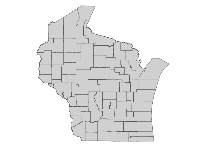
For example, we can find the polygon boundaries for all the counties in Wisconsin using the code below.
wisconsin <- counties(state = "Wisconsin") ## | | | 0% | | | 1% | |= | 1% | |= | 2% | |== | 2% | |== | 3% | |=== | 4% | |=== | 5% | |==== | 5% | |==== | 6% | |===== | 6% | |===== | 7% | |===== | 8% | |====== | 8% | |====== | 9% | |======= | 9% | |======= | 10% | |======== | 11% | |======== | 12% | |========= | 12% | |========= | 13% | |========== | 14% | |========== | 15% | |=========== | 15% | |=========== | 16% | |============ | 16% | |============ | 17% | |============ | 18% | |============= | 18% | |============= | 19% | |============== | 19% | |============== | 20% | |============== | 21% | |=============== | 21% | |=============== | 22% | |================ | 22% | |================ | 23% | |================= | 24% | |================= | 25% | |================== | 25% | |================== | 26% | |=================== | 26% | |=================== | 27% | |=================== | 28% | |==================== | 28% | |==================== | 29% | |===================== | 29% | |===================== | 30% | |===================== | 31% | |====================== | 31% | |====================== | 32% | |======================= | 32% | |======================= | 33% | |======================== | 34% | |======================== | 35% | |========================= | 35% | |========================= | 36% | |========================== | 36% | |========================== | 37% | |========================== | 38% | |=========================== | 38% | |=========================== | 39% | |============================ | 39% | |============================ | 40% | |============================ | 41% | |============================= | 41% | |============================= | 42% | |============================== | 42% | |============================== | 43% | |=============================== | 44% | |=============================== | 45% | |================================ | 45% | |================================ | 46% | |================================= | 46% | |================================= | 47% | |================================= | 48% | |================================== | 48% | |================================== | 49% | |=================================== | 49% | |=================================== | 50% | |=================================== | 51% | |==================================== | 51% | |==================================== | 52% | |===================================== | 52% | |===================================== | 53% | |===================================== | 54% | |====================================== | 54% | |====================================== | 55% | |======================================= | 55% | |======================================= | 56% | |======================================== | 56% | |======================================== | 57% | |======================================== | 58% | |========================================= | 58% | |========================================= | 59% | |========================================== | 59% | |========================================== | 60% | |========================================== | 61% | |=========================================== | 61% | |=========================================== | 62% | |============================================ | 62% | |============================================ | 63% | |============================================ | 64% | |============================================= | 64% | |============================================= | 65% | |============================================== | 65% | |============================================== | 66% | |=============================================== | 66% | |=============================================== | 67% | |=============================================== | 68% | |================================================ | 68% | |================================================ | 69% | |================================================= | 69% | |================================================= | 70% | |================================================= | 71% | |================================================== | 71% | |================================================== | 72% | |=================================================== | 72% | |=================================================== | 73% | |=================================================== | 74% | |==================================================== | 74% | |==================================================== | 75% | |===================================================== | 75% | |===================================================== | 76% | |====================================================== | 76% | |====================================================== | 77% | |====================================================== | 78% | |======================================================= | 78% | |======================================================= | 79% | |======================================================== | 79% | |======================================================== | 80% | |======================================================== | 81% | |========================================================= | 81% | |========================================================= | 82% | |========================================================== | 82% | |========================================================== | 83% | |========================================================== | 84% | |=========================================================== | 84% | |=========================================================== | 85% | |============================================================ | 85% | |============================================================ | 86% | |============================================================= | 86% | |============================================================= | 87% | |============================================================= | 88% | |============================================================== | 88% | |============================================================== | 89% | |=============================================================== | 89% | |=============================================================== | 90% | |================================================================ | 91% | |================================================================ | 92% | |================================================================= | 92% | |================================================================= | 93% | |================================================================== | 94% | |================================================================== | 95% | |=================================================================== | 95% | |=================================================================== | 96% | |==================================================================== | 96% | |==================================================================== | 97% | |==================================================================== | 98% | |===================================================================== | 98% | |===================================================================== | 99% | |======================================================================| 99% | |======================================================================| 100% tm_shape(wisconsin) + tm_polygons()
-
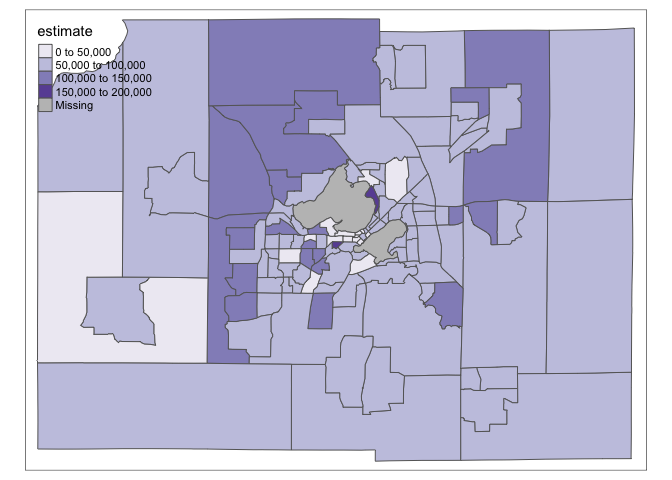
Similarly, we can create a choropleth of household income across all census extracts in Dane County retrieved in the previous step.
# sign up for an api key at http://api.census.gov/data/key_signup.html dane <- get_acs( state = "WI", county = "Dane", geography = "tract", variables = "B19013_001", # household income geometry = TRUE ) ## | | | 0% | |= | 2% | |== | 3% | |=== | 5% | |==== | 6% | |===== | 7% | |====== | 9% | |======= | 10% | |======== | 12% | |=========== | 15% | |============ | 16% | |============ | 17% | |============= | 19% | |============== | 20% | |=============== | 21% | |================ | 22% | |================ | 23% | |================== | 25% | |================== | 26% | |=================== | 27% | |==================== | 28% | |===================== | 29% | |====================== | 31% | |======================= | 32% | |======================== | 34% | |========================= | 36% | |========================== | 37% | |=========================== | 38% | |============================ | 40% | |============================= | 42% | |============================== | 43% | |=============================== | 44% | |================================ | 45% | |================================= | 47% | |================================= | 48% | |================================== | 48% | |================================== | 49% | |=================================== | 50% | |==================================== | 51% | |===================================== | 52% | |====================================== | 54% | |================================================= | 70% | |================================================== | 72% | |=================================================== | 73% | |==================================================== | 74% | |==================================================== | 75% | |===================================================== | 75% | |===================================================== | 76% | |====================================================== | 77% | |======================================================= | 78% | |======================================================== | 80% | |========================================================= | 81% | |========================================================= | 82% | |========================================================== | 82% | |=========================================================== | 84% | |============================================================ | 86% | |============================================================= | 87% | |=============================================================== | 90% | |================================================================ | 91% | |================================================================= | 93% | |================================================================== | 94% | |=================================================================== | 96% | |==================================================================== | 97% | |==================================================================== | 98% | |===================================================================== | 99% | |======================================================================| 100% tm_shape(dane) + tm_polygons(col = "estimate", palette = "Purples")
Transforming Projections
-
An important subtlety of geographic data visualization is that all our maps are in 2D, but earth is 3D. The process of associating points on the earth with 2D coordinates is called “projection.” All projections introduce some level of distortion, and there is no universal, ideal projection.
-
A common source of bugs is to use two different projections for the same analysis. In this class, we will always use the EPSG:4326 projection, which is what is used in most online maps. But in your own projects, you should always check that the projections are consistent across data sources. If you find an inconsistency, it will be important to “reproject” the data into the same CRS. Both
sfandterrahave utilities for supporting this.
Bivariate Choropleths
-
Choropleths are useful for encoding one data feature across a collection of polygons. If we have more than one feature of interest, there is often little we can do besides create several choropleths side-by-side, each with its own color scales. An important special case is when there are exactly two continuous variables of interest.
-
In this case, we can use something called a bivariate choropleth. This creates a two-dimensional color palette by blending a pair of color scales. Polygons are then encoded using this scheme. For example, in the example below, we can see the correlation structure between obesity adn diabetes across counties in the US.
health <- read_csv("../examples/week7/week7-3/cdc-diabetes-obesity.csv", na = "No Data") %>%
  mutate(
    diabetes_cat = cut(diabetes, 3),
    obesity_cat = cut(obesity, 3)
  )
us_counties <- counties() %>%
  mutate(county = str_c(STATEFP, COUNTYFP)) %>%
  filter(!(STATEFP %in% c("15", "02", "60", "66", "69", "72", "78"))) %>%
  left_join(health) %>%
  bi_class(x = diabetes_cat, y = obesity_cat, style = "quantile", dim = 3)

map <- us_counties %>%
  st_simplify(dTolerance = 1000) %>% # speeds up plot by coarsening
  ggplot() +
  geom_sf(aes(fill = bi_class), size = 0.1, show.legend = FALSE) +
  bi_scale_fill(pal = "GrPink", dim = 3) +
  bi_theme()

legend <- bi_legend(pal = "GrPink", dim = 3, xlab = "obesity", ylab = "diabetes")
map + inset_element(legend, 0, 0, .3, .3, align_to = "full")
Spatiotemporal Vis
- What if we have the spatial data measured over time? It is common to use faceting, with one facet per timepoint. However, this approach does not scale well when there are many timepoints of interest. Some have advocated for the use of time cubes, where a 2D map is repeated along a third time axis.

In this class though, we will steer away from 3D visualization. Instead, we will focus on approaches that leverage interactivity, specifically using animation or linked views. We’ll review some approaches next week.