Reading Data in D3

2022-06-01 00:00

Reading CSV files into javascript objects

These notes give an introduction to reading data into D3 scripts. The process is a bit different than read_csv in R, but the pattern described here can be used quite generally.
There is a function called d3.csv that at first might seem like a simple solution to reading in files. It would be great if we could write something like,
```
// this doesn't work!
let data = d3.csv("gapminder.csv")
console.log(data)
visualize(data)
```
where the function visualize does all the DOM manipulation to make the visualization.
Unfortunately, this approach does not work. The reason is that javascript is designed with reactive programming in mind, so code doesn’t necessarily run sequentially. We need to explicitly tell javascript to only run visualize after all the data has been read in. This can be accomplished using the .then() method,
```
 d3.csv("gapminder.csv")
   .then(data => console.log(data))
```
On some browsers, you can now navigate to the HTML page that includes this script, and the data will be loaded. But on many modern browsers, you will see an error like this in the console,
```
 Access to fetch at 'file:///Users/ksankaran/Desktop/teaching/stat679_code/examples/week5/week5-3/gapminder.csv' from origin 'null' has been blocked by CORS policy: Cross origin requests are only supported for protocol schemes: http, data, chrome, chrome-extension, chrome-untrusted, https.
```
The browser is trying to protect us from downloading a file from a suspicious link. To resolve this, we need to run our own server. From your terminal, go to the directory with the HTML page you want to run. Then, execute,
```
 python3 -m http.server
```
You should see a message like,
```
 Serving HTTP on :: port 8000 (http://[::]:8000/) ...
```
If you go the page with the port number in the message (http://localhost:8000 in the example here), you should see your HTML page. When you click on that page, you will no longer see the data loading error — the file is now trusted for download.
You should now be able to see the data in the console,

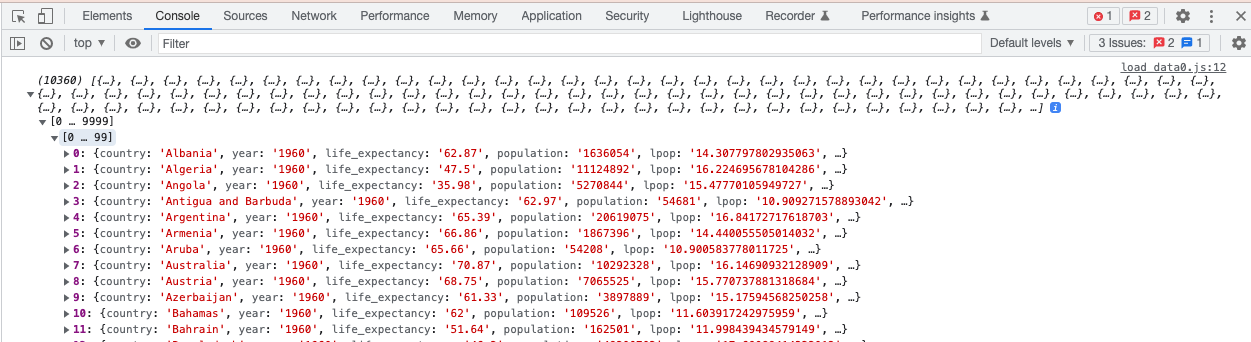
We are almost ready for visualization! But there is still one detail we should account for. If we look closely, we can see that all the numbers are being read in as character strings. We need to parse these into numbers before they can be used.
d3.csv can take as an argument a function to modify each row of the csv as it is being read in. This is handy in case we want to manually change the types of object items as they are read in. We will usually not have to do this work ourselves – we can rely on a built in function, d3.autoType, to automatically recognize the number columns in the CSV. Using this function in d3.csv, we now see a version of the data with numbers correctly parsed.
```
 d3.csv("gapminder.csv", d3.autoType)
   .then(data => console.log(data));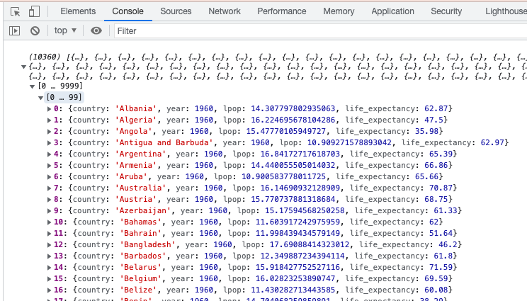
```
We are now done with loading data in D3. The main ideas are,
- Data can’t be easily read into local variables, like in R. Instead, use .then().
- To ensure the data are not blocked by the browser, we need to start a backend server with python3 -m http.server.
- Numeric variables need to be parsed using d3.autoType.
Since we’ve gone through all the work of reading in these data, let’s make a quick visualization. Let’s visualize log population, lpop, against life expectancy, life_expectancy, for the year 1965. We first filter the data to this year,
```
  data = data.filter(d => d.year == 1965)
```
Next, we will bind a circle for each country in the filtered array. We create a selection of circles on the parent SVG and bind the data,
```
d3.select("svg")
  .selectAll("circle")
  .data(data)
```
Since there are not yet any HTML tags in this selection, we can refer to each array element using .enter(). The next .append() line draws each of these entered elements.
```
d3.select("svg")
  .selectAll("circle")
  .data(data).enter()
  .append("circle")
```
We then set the cx and cy coordinates for all circles on the page. I’ve multiplied the log population by 10, since cx is specified in terms of pixel coordinates. Since log populations are all relatively small, the points would all overlap if I didn’t manually multiply them like this.
```
d3.select("svg")
  .selectAll("circle")
  .data(data).enter()
  .append("circle")
  .attrs({
    cx: d => 10 * d.lpop,
    cy: d => d.life_expectancy,
    r: 2
   })
```

Finally, we wrap this block into a single function which is called as soon as the data are loaded.

function visualize(data) {
  data = data.filter(d => d.year == 1965)
  d3.select("svg")
    .selectAll("circle")
    .data(data).enter()
    .append("circle")
    .attrs({
      cx: d => 10 * d.lpop,
      cy: d => d.life_expectancy,
      r: 2
     })
}

d3.csv("gapminder.csv", parse_row)
  .then(visualize);

The result is very primitive looking, but it does use a real dataset. We’ll revisit these data in the next lecture to see how we can support more realistic visual queries.

Statistical Data Visualization