Topic modeling is a type of dimensionality reduction method that is especially useful for high-dimensional count matrices. For example, it can be applied to,
- Text data analysis, where each row is a document and each column is a word. The \(ij^{th}\) entry contains the count of the \(j^{th}\) word in the \(i^{th}\) document.
- Gene expression analysis, where each row is a biological sample and each column is a gene. The \(ij^{th}\) entry measures the amount of gene \(j\) expressed in sample \(i\).
For clarity, we will refer to samples as documents and features as words. However, keep in mind that these methods can be used more generally – we will see a biological application three lectures from now.
These models are useful to know about because they provide a compromise between clustering and PCA.
- In clustering, each document would have to be assigned to a single topic. In contrast, topic models allow each document to partially belong to several topics simultaneously. In this sense, they are more suitable when data do not belong to distinct, clearly-defined clusters.
- PCA is also appropriate when the data vary continuously, but it does not provide any notion of clusters. In contrast, topic models estimate \(K\) topics, which are analogous to a cluster centroids (though documents are typically a mix of several centroids).
Without going into mathematical detail, topic models perform dimensionality reduction by supposing,
- Each document is a mixture of topics.
- Each topic is a mixture of words.

Figure 1: An overview of the topic modeling process. Topics are distributions over words, and the word counts of new documents are determined by their degree of membership over a set of underlying topics. In an ordinary clustering model, the bars for the memberships would have to be either pure purple or orange. Here, each document is a mixture.
To illustrate the first point, consider modeling a collection of newspaper articles. A set of articles might belong primarily to the “politics” topic, and others to the “business” topic. Articles that describe a monetary policy in the federal reserve might belong partially to both the “politics” and the “business” topic.
For the second point, consider the difference in words that would appear in politics and business articles. Articles about politics might frequently include words like “congress” and “law,” but only rarely words like “stock” and “trade.”
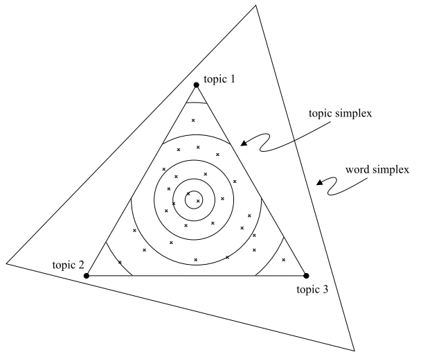
Geometrically, LDA can be represented by the following picture. The corners of the simplex1 represent different words (in reality, there would be \(V\) different corners to this simplex, one for each word). A topic is a point on this simplex. The closer the topic is to one of the corners, the more frequently that word appears in the topic.

Figure 2: A geometric interpretation of LDA, from the original paper by Blei, Ng, and Jordan.
- A document is a mixture of topics, with more words coming from the topics that it is close to. More precisely, a document that is very close to a particular topic has a word distribution just like that topic. A document that is intermediate between two topics has a word distribution that mixes between both topics. Note that this is different from a clustering model, where all documents would lie at exactly one of the corners of the topic simplex. Finally, note that the topics form their own simplex, since each document can be described as a mixture of topics, with mixture weights summing up to 1.
A simplex is the geometric object describing the set of probability vectors over \(V\) elements. For example, if \(V = 3\), then \(\left(0.1, 0, 0.9\right)\) and \(\left(0.2, 0.3, 0.5\right)\) belong to the simplex, but not \(\left(0.3, 0.1, 9\right)\), since it sums to a number larger than 1.↩︎