- High-dimensional data are data where many features are collected for each observation. These tend to be wide datasets with many columns. The name comes from the fact that each row of the dataset can be viewed as a vector in a high-dimensional space (one dimension for each feature). These data are common in modern applications,
- Each cell in a genomics dataset might have measurements for hundreds of molecules.
- Each survey respondent might provide answers to dozens of questions.
- Each image might have several thousand pixels.
- Each document might have counts across several thousand relevant words.
For low-dimensional data, we could visually encode all the features in our data directly, either using properties of marks or through faceting. In high-dimensional data, this is no longer possible.
However, though there are many features associated with each observation, it may still be possible to organize samples across a smaller number of meaningful, derived features.
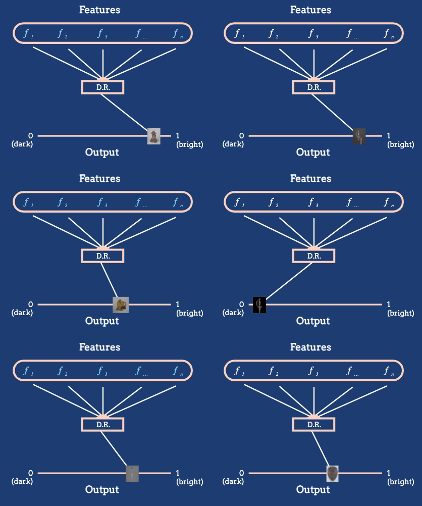
For example, consider the Metropolitan Museum of Art dataset, which contains images of many artworks. Abstractly, each artwork is a high-dimensional object, containing pixel intensities across many pixels. But it is reasonable to derive a feature based on the average brightness.

Figure 1: An arrangement of artworks according to their average pixel brightness, as given in the reading.
- In general, manual feature construction can be difficult. Algorithmic approaches try streamline the process of generating these maps by optimizing some more generic criterion. Different algorithms use different criteria, which we will review in the next couple of lectures.

Figure 2: The dimensionality reduction algorithm in this animation converts a large number of raw features into a position on a one-dimensional axis defined by average pixel brightness. In general, we might reduce to dimensions other than 1D, and we will often want to define features tailored to the dataset at hand.
- Informally, the goal of dimensionality reduction techniques is to produce a low-dimensional “atlas” relating members of a collection of complex objects. Samples that are similar to one another in the high-dimensional space should be placed near one another in the low-dimensional view. For example, we might want to make an atlas of artworks, with similar styles and historical periods being placed near to one another.