Vector Data

Manipulating and visualizing spatial vector data.

Reading, Recording, Rmarkdown

library(ceramic)
library(knitr)
library(sf)
library(spData)
library(tidyverse)
library(tmap)
theme_set(theme_minimal())

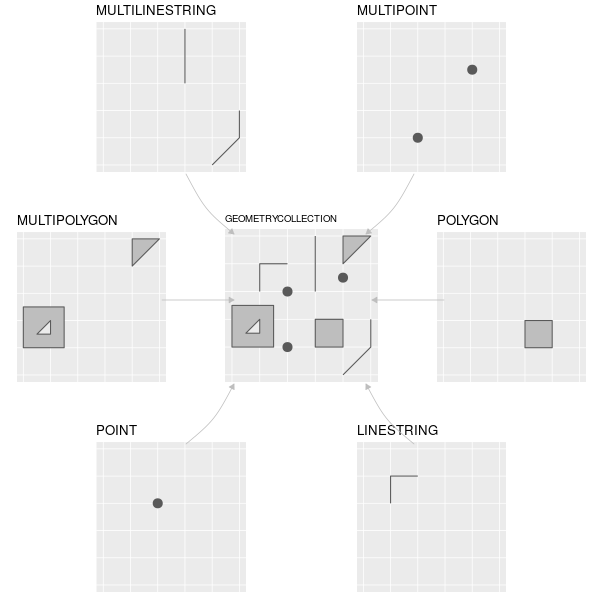
1. As mentioned previously, vector data are used to store geometric spatial data. Specifically, there are 7 types of geometric information that are commonly used, as given in the figure below.

include_graphics("https://krisrs1128.github.io/stat479/posts/2021-03-02-week7-2/sf-classes.png")

3. We can construct these geometric objects from scratch. For example, starting from the defining coordinates, we can use st_point to create a point object,

# make a point
p <- st_point(c(5, 2))
plot(p)

st_linestring to create a linestring,

# make a line
linestring_matrix <- rbind(c(1, 5), c(4, 4), c(4, 1), c(2, 2), c(3, 2))
p <- st_linestring(linestring_matrix)
plot(p)

and st_polygon to create a polygon.

# make a polygon
polygon_list <- list(rbind(c(1, 5), c(2, 2), c(4, 1), c(4, 4), c(1, 5)))
p <- st_polygon(polygon_list)
plot(p)

4. Different geometries can be combined into a geometry collection, using sfc.

point1 <- st_point(c(5, 2))
point2 <- st_point(c(1, 3))
points_sfc <- st_sfc(point1, point2)
plot(points_sfc)

5. Real-world vector datasets are more than just these geometries — they also associate each geometry with some additional information about each feature. We can add this information to the geometries above by associating each element with a row of a data.frame. This merging is accomplished by st_sf, using geometry to associate a raw st_geom each row of a data.frame.

lnd_point <- st_point(c(0.1, 51.5))                
lnd_geom <- st_sfc(lnd_point, crs = 4326)         
lnd_attrib = data.frame(                        
  name = "London",
  temperature = 25,
  date = as.Date("2017-06-21")
  )

lnd_sf = st_sf(lnd_attrib, geometry = lnd_geom)

Visualization

5. Vector data can be directly plotted using base R. For example, suppose we want to plot the boundaries of India, within it’s local context. We can use the world dataset, provided by the spData package. Each row of the world object contains both the boundary of a country (in the geom column) and information about its location and population characteristics.

data(world)
head(world)

Simple feature collection with 6 features and 10 fields
Geometry type: MULTIPOLYGON
Dimension:     XY
Bounding box:  xmin: -180 ymin: -18.28799 xmax: 180 ymax: 83.23324
Geodetic CRS:  WGS 84
# A tibble: 6 x 11
  iso_a2 name_long      continent   region_un subregion type  area_km2
  <chr>  <chr>          <chr>       <chr>     <chr>     <chr>    <dbl>
1 FJ     Fiji           Oceania     Oceania   Melanesia Sove~   1.93e4
2 TZ     Tanzania       Africa      Africa    Eastern ~ Sove~   9.33e5
3 EH     Western Sahara Africa      Africa    Northern~ Inde~   9.63e4
4 CA     Canada         North Amer~ Americas  Northern~ Sove~   1.00e7
5 US     United States  North Amer~ Americas  Northern~ Coun~   9.51e6
6 KZ     Kazakhstan     Asia        Asia      Central ~ Sove~   2.73e6
# i 4 more variables: pop <dbl>, lifeExp <dbl>, gdpPercap <dbl>,
#   geom <MULTIPOLYGON [arc_degree]>

This makes the plot, using dplyr to filter down to just the row containing the India geometry.

india_geom <- world %>%
  filter(name_long == "India") %>%
  st_geometry()

plot(india_geom)

6. Using base R, we can also layer on several vector objects, using add = TRUE.

world_asia <- world %>%
  filter(continent == "Asia")

plot(india_geom, expandBB = c(0, 0.2, 0.1, 1), col = "gray", lwd = 3)
plot(st_union(world_asia), add = TRUE)

7. We can also use tm_polygons in tmap. To change the coordinates of the viewing box, we can set the bbox (bounding box) argument.

bbox <- c(60, 5, 110, 40)
tm_shape(world_asia, bbox = bbox) +
  tm_polygons(col = "white") +
  tm_shape(india_geom) +
  tm_polygons()

8. We can also encode data that’s contained in the vector dataset.

tm_shape(world_asia, bbox = bbox) +
  tm_polygons(col = "lifeExp") +
  tm_polygons()

9. Even in this more complex setup, where we work with background images and vector data rather than standard data.frames, we can still apply the kinds of visual encoding ideas that we are familiar with. For example, we can still color code or facet by fields in the vector dataset. To illustrate, we revisit the bus route data from the last lecture and distinguish between buses operated by the cities of Madison vs. Monona. Before plotting, we fetch the underlying data.

Sys.setenv(MAPBOX_API_KEY="pk.eyJ1Ijoia3Jpc3JzMTEyOCIsImEiOiJjbDYzdjJzczQya3JzM2Jtb2E0NWU1a3B3In0.Mk4-pmKi_klg3EKfTw-JbQ")
basemap <- cc_location(loc= c(-89.401230, 43.073051), buffer = 15e3)
bus <- read_sf("https://uwmadison.box.com/shared/static/5neu1mpuh8esmb1q3j9celu73jy1rj2i.geojson")

tm_shape(basemap) +
  tm_rgb() +
  tm_shape(bus) +
  tm_lines(col = "#bc7ab3", size = 1)

Note that operator is the field containing information about which city is operating the buses. We can color code the routes by this attribute.

tm_shape(basemap) +
  tm_rgb() +
  tm_shape(bus) +
  tm_lines(col = "operator", size = 1) +
  tm_layout(legend.bg.color = "white")

Alternatively, we can facet.

tm_shape(basemap) +
  tm_rgb() +
  tm_shape(bus) +
  tm_lines(col = "operator", size = 1) +
  tm_facets("operator")