- There could probably be an entire class taught on the history of data
visualization. The reason it is worth covering in an otherwise
practically-oriented class is that,
- Historical study can illuminate the core intellectual foundation on which the entire discipline of data visualization is built.
- The limits, biases, and trends of our current era become clear when considering it within its full historical context.
- It’s often possible to draw inspiration from past masters.
- It can be humbling to realize that now-commonplace ideas had to be discovered. If it took until 1833 until the first scatterplot was published, then what ideas have we yet to find?
- The reading divides up the history of data visualization into 8 epochs. In these notes, we will consider the 5 epochs before 1900.
Before 1600: Early Maps and Diagrams
- It might come as a surprise, but visualization has been around since the invention of writing. The Egyptians made maps, and there are examples multiple time series plots from the 10th century.

Figure 1: Possibly the earliest multiple time series visualization, showing the movement of various planets, from In Somnium Scripionus.
- However, most visualizations were focused on physical geographical or astronomical quantities, and even these quantities were only imprecisely measured. Without more formal data gathering instruments, there could not be much data visualization.
1600 - 1700: Measurement and Theory
- The situation begins to change around 1600, at the dawn of the scientific revolution. All of a sudden, precise measurement of physical space become possible. Also, important new mathematical ideas were introduced, like probability, calculus, and reasoning about functions. This created the right environment for the design of some of the first truly sophisticated data visualizations, like
- Christopher Scheiner’s 1630 visualization of sunspots over time (a first instance of faceting),

Figure 2: Scheiner’s visualization of sunspots, which played a role in his dialogues with Galileo.
- Edmond Halley’s plot of barometric pressure against altitude (an first instance of one feature being plotted against another), and

Figure 3: One of the first bivariate plots, relating barometric pressure to altitude. Note that absence of the true observed data.
- Edmond Halley’s plot of wind speed over the ocean (a first visualization of a vector field).
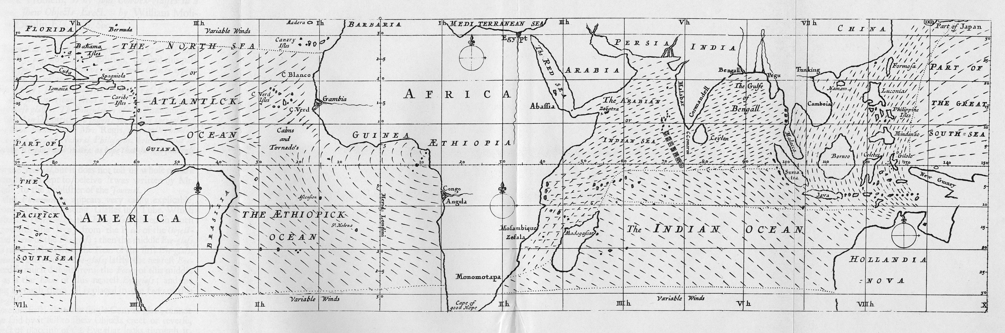
Figure 4: A plot of trade winds, appearing in An Historical Account of the Trade Winds, and Monsoons, Observable in the Seas between and near the Tropicks, with an Attempt to Assign the Phisical Cause of the Said Wind.
- During this period, the scientific value of visual thinking was more or less established. However, there were still only relatively few graphical forms available, and the focus continued to remain on visualizing physical quantities, rather than more general social, economic, biological, or ecological data.
1700 - 1800
During this period, many new graphical forms were invented, including timelines, cartograms, functional interpolations, line graphs, bar charts, and pie charts. Further, forms from earlier, like maps and function plots, became more firmly established.
This was also when three-color printing was invented. Before this point, color could not be used as an encoding channel.
In this century, governments also began large-scale data collection of social and economic statistics1. One of the most prolific inventors of data visualizations, William Playfair2, was used visualization to study a variety of economic problems. In addition to inventing line, bar, and pie charts, he experimented with original ways of composing multiple graphs to suggest the relationships between variables.

Figure 5: One of William Playfair’s data visualizations, juxtaposing the price of wheat with growth in wages.
1800 - 1850
This was a period of maturation for the field of data visualization. By this point, visualization had become standard in scientific publications. Advances in printing technology also made it also became easier to mass produce visualizations.
It was also around this time that the scope of problems studied through visualization expanded far beyond display of purely physical (geographical and astronomical) applications. Two areas in particular flourished, applications to social science and to engineering.
- Visualization in the social sciences began to emerged in response to government sponsored collection of social statistics – data about crime, births, and deaths, among other topics. This wasn’t a purely intellectual exercise: understanding demographic trends was important for countries that were often at war with another.
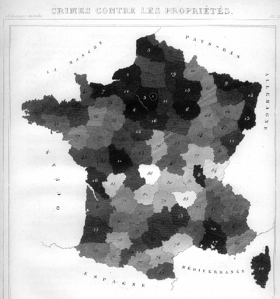
Figure 6: A visualization of property crime statistics, by Andre-Michel Guerry (1829).
- In engineering, the idea that visualization could serve as a computational aid become more and more common. For example, rather the chart below, by Charles Joseph Minard, displays the cost of transporting goods across different stretches of a canal. Vertical breaks correspond to cities along the canal, and the area of the square between cities encodes the cost of transportation between those cities. While the information could be stored in a table, it becomes easier to perform mental computations (and make guesstimates) using the display.

Figure 7: Minard’s 1844 visualization of the transport costs across the Canal du Centre in France.
1850 - 1900: The Golden Age
It might be counterintuitive that there was a golden age of visualization a century before the first computers were invented. However, a look at the visualizations from this period demonstrate that this was a period where visualizations inspired scientific discoveries, informed commercial decisions, and guided social reform.
For example, in public health, Florence Nightingale invented new visualizations to demonstrate the impact of sanitary practices in hospital-induced infections and death. Similarly, it was a visualization that guided John Snow to the source of the 1855 cholera epidemic.

Figure 8: Florence Nightingale’s visualization of hospital mortality statistics from the Crimean War, used to support a campaign for sanitary reforms.
- Some of the graphical innovations include,
- 3D function plots. The plot below, by Luigi Perozzo, shows population size broken down into age groups and traced over time.

Figure 9: Luigi Perrozo’s 1879 3D visualizations of population over time.
- Flow diagrams. Charles-Joseph Minard, who we met before with the canal visualization, was a master of these displays. One in particular is widely considered a masterpiece, it shows the size of Napoleon’s army during it’s Russian Campaign.

Figure 10: Minard’s flow display of the size of Napoleon’s army during the Russia Campaign.
- Multivariate visualization. Francis Galton made some of the first efforts to visualize more than 3 variables at a time. His Meteorographica, published in 1863, contained over 600 visualizations of weather data that had been collected for decades, but never visualized. One plot, shown below, led to the discovery of anticyclones.

Figure 11: Galton’s display of weather patterns. Low pressure (black) areas tend to have clockwise wind patterns, while high pressure (red) tends to have anticlockwise wind patterns.
- This was also an age of state-sponsored atlases. More than sponsoring the collection of data, governments assembled teams to visualize the results for official publication. From 1879 to 1897, the French Ministry of Public Works published the Albums de Statistique Graphique, which under the guidance of Émile Cheysson, developed some of the most imaginative and ambitious visualizations of the era.

Figure 12: A visualization of the flow of passengers and goods through railways from Paris. Each square shows the breakdown to cities further away, and color encodes the railines.