One of the fundamental principles in statistics is that, no matter how the experiment / study was conducted, if we ran it again, we would get different results. More formally, sampling variability creates uncertainty in our inferences.
How should we think about sampling variability in the context of clustering? This is a tricky problem, because you can permute the labels of the clusters without changing the meaning of the clustering. However, it is possible to measure and visualize the stability of a point’s cluster assignment.
To make this less abstract, consider an example. A study has found a collection of genes that are differentially expressed between patients with two different subtypes of a disease. There is an interest in clustering genes that have similar expression profiles across all patients — these genes probably belong to similar biological processes.
Once you run the clustering, how sure can you be that, if the study would run again, you would recover a similar clustering? Are there some genes that you are sure belong to a particular cluster? Are there some that lie between two clusters?
To illustrate, consider the simulated dataset below. Imagine that the rows are patients, the column are genes, and the colors are the expression levels of genes within patients. There are 5 clusters of genes here (columns 1 - 20 are cluster 1, 21 - 41 are cluster 2, …). The first two clusters are only weakly visible, while the last three stand out strongly.
n_per <- 20
p <- n_per * 5
Sigma1 <- diag(2) %x% matrix(rep(0.3, n_per ** 2), nrow = n_per)
Sigma2 <- diag(3) %x% matrix(rep(0.6, n_per ** 2), nrow = n_per)
Sigma <- bdiag(Sigma1, Sigma2)
diag(Sigma) <- 1
mu <- rep(0, 100)
x <- mvrnorm(25, mu, Sigma)

cols <- c('#f6eff7','#bdc9e1','#67a9cf','#1c9099','#016c59')
superheat(
  x,
  pretty.order.rows = TRUE,
  bottom.label = "none",
  heat.pal = cols,
  left.label.text.size = 3,
  legend = FALSE
)
Figure 1: A simulated clustering of genes (columns) across rows (patients).
- The main idea for how to compute cluster stability is to bootstrap (i.e., randomly resample) the patients and see whether the cluster assignments for each gene change. More precisely, we use the following strategy,
- Using all the patients, \(X\), estimate the cluster centroids \(c_{1}, \dots, c_{K}\).
- For \(B\) bootstrap iterations, perform the following.
- Sample the patients with replacement, generating a bootstrap resampled version of the dataset \(X_{b}^{\ast}\).
- Permute the original cluster centroids to reflect the order of patients in \(X_{b}^{\ast}\). Call the permuted centroids \(c_{1b}^{\ast}, \dots, c_{Kb}^{\ast}\).
- Assign genes in \(X_{b}^{\ast}\) to the cluster \(k\) of the closest \(c_{bk}^{\ast}\).
- We quantify our certainty that gene \(j\) belongs to cluster \(k\) by counting the number of times that gene \(j\) was assigned to cluster \(k\).
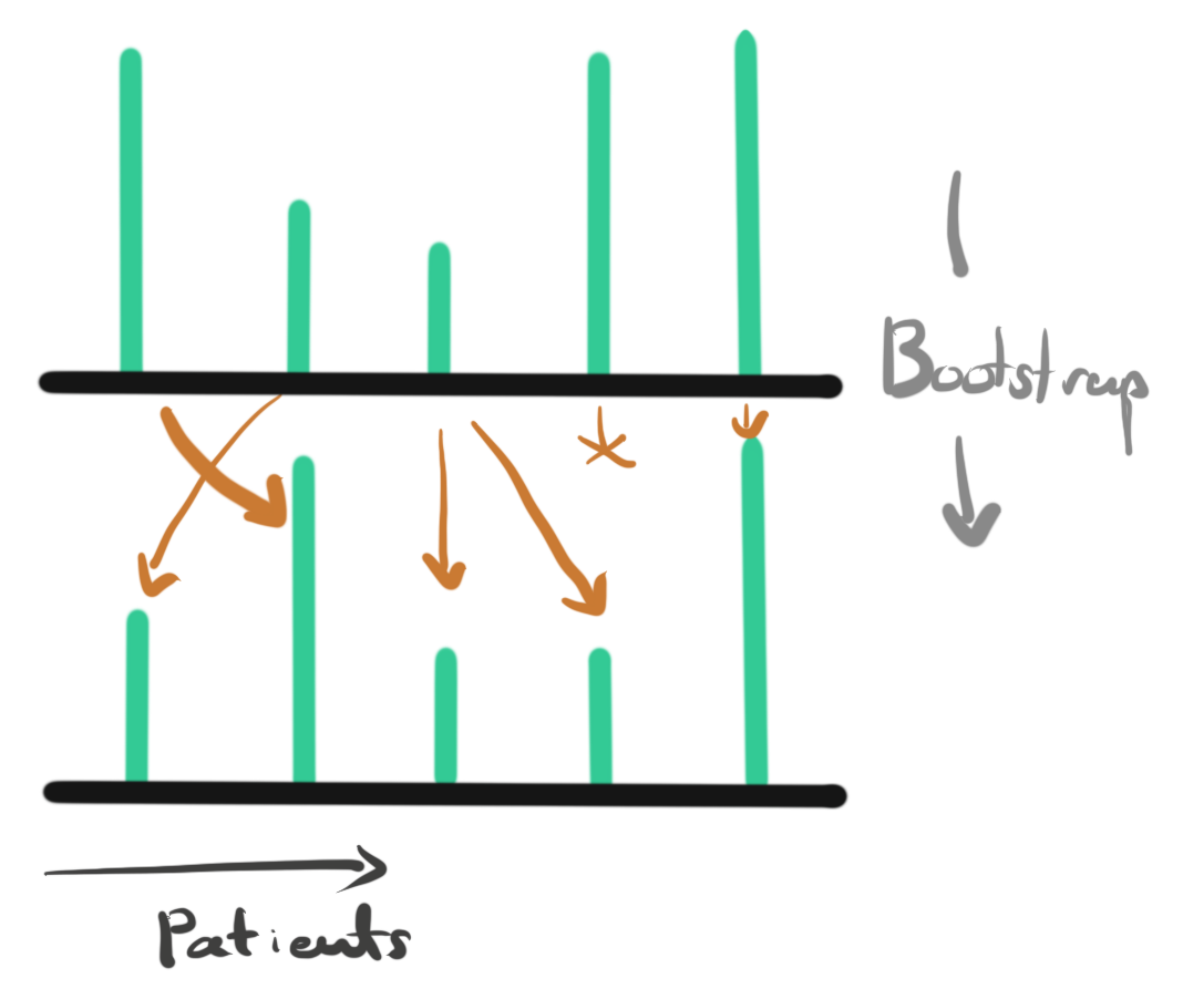
- The picture below describes the bootstrapping process for a gene. The two rows correspond to the original and bootstrapped representations a specific gene, respectively. Each bar gives the expression level of the gene for one individual. Due to the random sampling in the bootstrapped dataset, some individuals become overrepresented and some are removed. If we also permute the centroids in the same way, we get a new distance between genes and their centroids. Since the patients who are included changes, the distances between each gene and each centroid changes, so the genes might be assigned to different clusters.

K <- 5
B <- 1000
cluster_profiles <- kmeans(t(x), centers = K)$centers
cluster_probs <- matrix(nrow = ncol(x), ncol = B)

for (b in seq_len(B)) {
  b_ix <- sample(nrow(x), replace = TRUE)
  dists <- as.matrix(pdist(t(x[b_ix, ]), cluster_profiles[, b_ix]))
  cluster_probs[, b] <- apply(dists, 1, which.min)
}

cluster_probs <- as_tibble(cluster_probs) %>%
  mutate(gene = row_number()) %>%
pivot_longer(-gene, names_to = "b", values_to = "cluster")- The table below shows the result of this procedure. In each bootstrap iteration, gene 1 was assigned to cluster 4, so we can rely on that assignment. On the other hand, gene 3 is assigned to cluster 4 75% of the time, but occasionally appears in clusters 1, 2, and 5.
cluster_probs <- cluster_probs %>%
  mutate(cluster = as.factor(cluster)) %>%
  group_by(gene, cluster) %>%
  summarise(prob = n() / B)

cluster_probs
# A tibble: 267 × 3
# Groups: gene [100]
gene cluster prob
<int> <fct> <dbl>
1 1 2 0.956
2 1 3 0.041
3 1 5 0.003
4 2 2 0.778
5 2 5 0.222
6 3 1 0.001
7 3 2 0.978
8 3 5 0.021
9 4 1 0.001
10 4 2 0.689
# … with 257 more rows- These fractions for all genes are summarized by the plot below. Each row is a gene. The length of each color gives the number of times that gene was assigned to that cluster. The genes from rows 41 - 100 are all clearly distinguished, which is in line with what we saw visually in the heatmap above. The first two clusters are somewhat recovered, but since they were often assigned to alternative clusters, we can conclude that they were harder to demarcate out than the others.
ggplot(cluster_probs) +
  geom_bar(aes(y = as.factor(gene), x = prob, col = cluster, fill = cluster), stat = "identity") +
  scale_fill_brewer(palette = "Set2") +
  scale_color_brewer(palette = "Set2") +
  scale_x_continuous(expand = c(0, 0)) +
  labs(y = "Gene", x = "Proportion") +
  theme(
    axis.ticks.y = element_blank(),
    axis.text.y = element_text(size = 7),
    legend.position = "bottom"
  )