Visualize Time Series Heatmaps

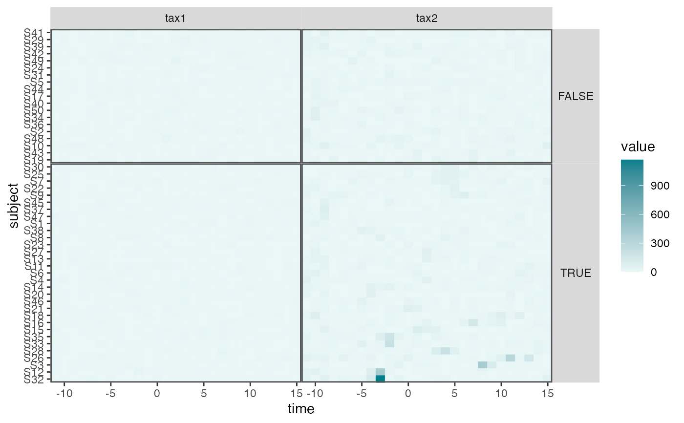
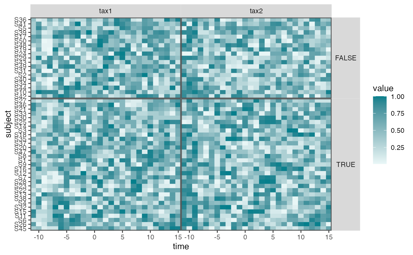
This is a helper function to visualize time series for a subset of taxa across all subjects. It is used in the raw data figures in the case studies section of the accompanying manuscript.

Usage

interaction_hm(values_df, taxa, condition = NULL, r = 0, ...)

Arguments

values_df

A data.frame containing joined information from a ts_inter object. Each row should be one count from one taxon/subject pair. The output of pivot_ts reshape data to this format.

taxa

A character vector of taxa to filter down to in the final visualization.

condition

A subject-level variable to use during faceting. Defaults to no faceting.

r

When ordering subjects, we consider averages after rounding timepoints into bins. Large r corresponds to fine-grained binning, negative r are more coarse bins. Defaults to 0. See subject_order for details.

Examples

library(dplyr)
#> 
#> Attaching package: ‘dplyr’
#> The following objects are masked from ‘package:stats’:
#> 
#>     filter, lag
#> The following objects are masked from ‘package:base’:
#> 
#>     intersect, setdiff, setequal, union
data(sim_ts)
pivoted <- sim_ts |>
  pivot_ts() |>
  mutate(v_pos = V1 > 0)
#> Joining with `by = join_by(sample)`
#> Joining with `by = join_by(sample)`
#> Joining with `by = join_by(subject)`
interaction_hm(pivoted, c("tax1", "tax2"), "v_pos")


pivoted |>
  group_by(taxon) |>
  mutate(value = rank(value) / n()) |>
  interaction_hm(c("tax1", "tax2"), "v_pos")