Visualizing Mapping Models: Data Preparation

In these notes, we generate and visualize patches of data that will be used to train the mapping model. This is necessary for a few different reasons,

Preprocessing: The different channels need to be normalized, since they have such different ranges. There are also a few channels that we should drop, like the BQA quality channel we saw earlier.
Imbalance: The glaciers only make up a relatively fraction of the total area that we have imagery for. Our model can be trained more efficiently by zooming into the parts of the region that actually have glaciers.
Image size: Even if we completed these preprocessing steps, each satellite image is much larger than anything a machine learning algorithm could work with. We’ll need to break the processed imagery into pieces that can be sequentially streamed in for training the model¹

We load quite a few libraries for this step. Many will be familiar from the previous notes, but two new ones are abind, which is used to manipulate subsetted arrays of imagery, and reticulate, which is used to navigate back and forth between R and python. We need reticulate because we will save our final dataset as a collection of .npy numpy files – these are a convenient format for training our mapping model, which is written in python.

library("RStoolbox")
library("abind")
library("dplyr")
library("gdalUtils")
library("ggplot2")
library("gridExtra")
library("purrr")
library("raster")
library("readr")
library("reticulate")
library("sf")
library("stringr")
library("tidyr")

# setting up python environment
use_condaenv("notebook")
np <- import("numpy")
source("data.R")
theme_set(theme_minimal())
set.seed(123)

We want to make sure we don’t overfit to any particular region. To this end, we’ll use different geographic sub-basins for training and evaluation. For training, we’re just using the Kokcha basin, and for evaluation, we use Dudh Koshi. In general, our notebook takes arbitrary lists of basins, specified by links to csv files through the basins parameter in the header. In practice, a larger list of training basins would be used to train the model, but working with that is much more computationally intensive.

y_path <- file.path(params$raw_dir, "glaciers_small.geojson")
basins <- read_csv(params$basins)

y <- read_sf(y_path) %>%
  filter(Sub_basin %in% basins$Sub_basin)

To address the imbalance and image size issues, we’ll sample locations randomly from within the current basins’ glaciers. This is done using the st_sample function. More patches will translate into more patches for training the model, but it will also increase the chance that training patches overlap. You will see a warning message about st_intersection – it’s safe to ignore that for our purpose (we are ignoring the fact that the surface of the earth is slightly curved).

centers <- y %>%
  st_sample(params$n_patches, type = "random", by_polygon = FALSE) %>%
  st_coordinates()
colnames(centers) <- c("Longitude", "Latitude")

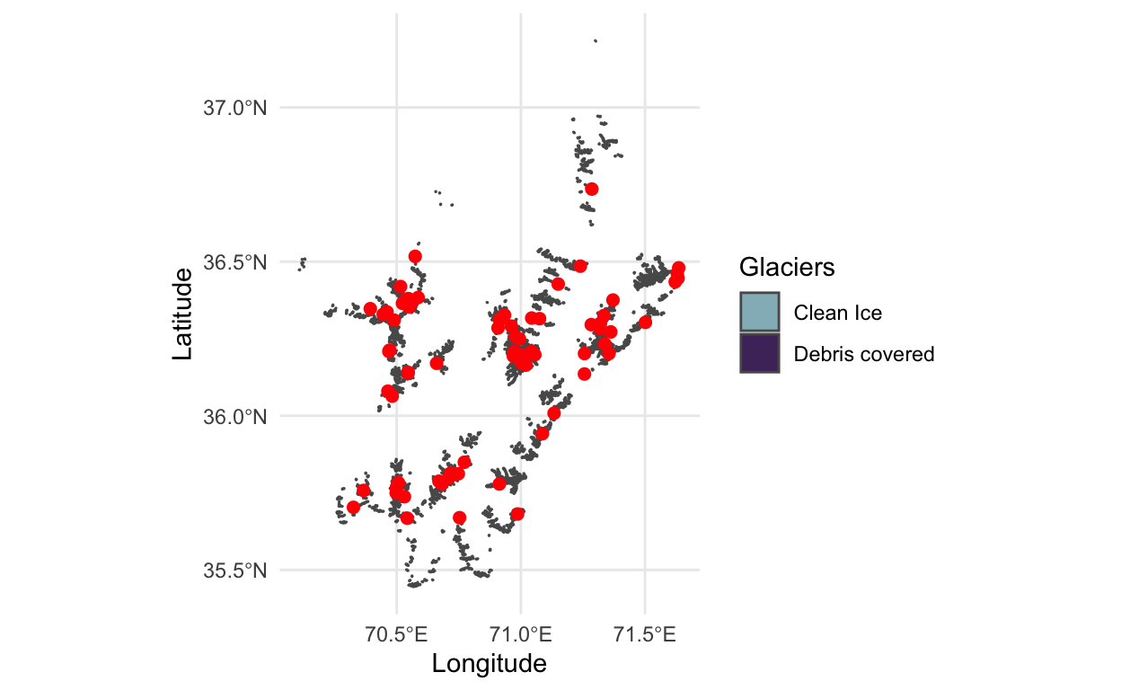
To better understand this sampling procedure, let’s visualize the centers of the sampled locations on top of the basins that are available for training. We can see that we have more samples in areas that have higher glacier density, which helps alleviate the imbalance problem. As an aside, this visualization gives an example of visualizing a spatial geometry (the glaciers object, y) together with an ordinary data frame (the centers for sampling).

p <- ggplot(y, aes(x = Longitude, y = Latitude)) +
  geom_sf(data = y, aes(fill = Glaciers)) +
  geom_point(data = as.data.frame(centers), col = "red", size = 2) +
  scale_fill_manual(values = c("#93b9c3", "#4e326a"))

p

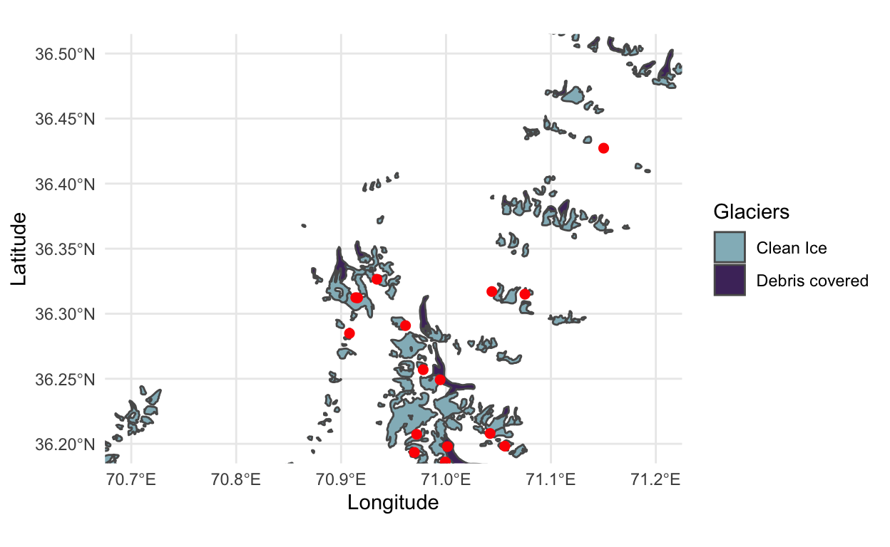
That image is quite zoomed out. To see some of the sampling locations along with just a few glaciers, we can zoom in, using the coord_sf modifier.

p + coord_sf(xlim = c(70.7, 71.2),  ylim = c(36.2, 36.5))

Now that we know where we want to sample our training imagery, let’s extract a patch. This is hidden away in generate_patch in the data.R script accompanying this notebook. This function also does all the preprocessing that we mentioned in the introduction. We’ll see the effect of this preprocessing in a minute – for now, let’s just run the patch extraction code. Note that we simultaneously extract a corresponding label, stored in patch_y. It’s these preprocessed satellite imagery - glacier label pairs that we’ll be showing to our model in order to train it.

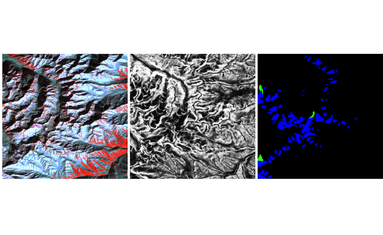
vrt_path <- file.path(params$raw_dir, "region.vrt")
ys <- y %>% split(.$Glaciers)

Let’s take a look at the preprocessed patches, just as a sanity check. We’re plotting the first of the sampled patches below. The image is much smaller now, but still contains a fair amount of glacier. Notice the false negative debris-covered glacier along the top of the image! A more sophisticated model would account for these kinds of data-specific variations, which become obvious when you visualize the data, but which are otherwise very hard to recognize.

patch <- generate_patch(vrt_path, centers[5, ])
patch_y <- label_mask(ys, patch$raster)
p <- list(
  plot_rgb(brick(patch$x), c(5, 4, 2), r = 1, g = 2, b = 3),
  plot_rgb(brick(patch$x), rep(13, 3)),
  plot_rgb(brick(patch_y), r = NULL)
)
grid.arrange(grobs = p, ncol = 3)

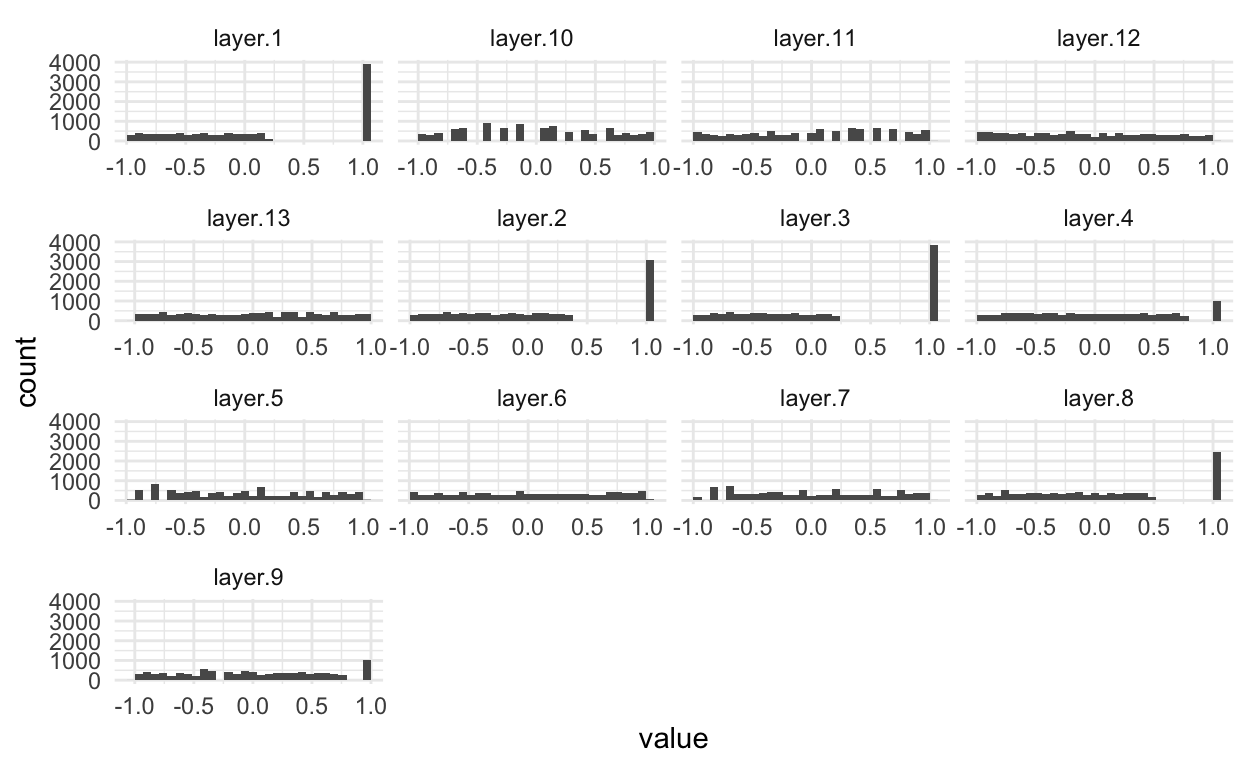
The other major change in these preprocessed images is that we’ve applied a linear transformation to each channel, mapping the sensor measurements to between \(\left[-1, 1\right]\) for every image. We’re using the same histogram code that we used in the first notebook.

sample_ix <- sample(nrow(patch$x), 100)
x_df <- patch$x[sample_ix, sample_ix, ] %>%
  brick() %>%
  as.data.frame() %>%
  pivot_longer(cols = everything())

ggplot(x_df) +
  geom_histogram(aes(x = value)) +
  facet_wrap(~ name, scale = "free_x")

Now that we’ve checked one of the patches, we can write them all to numpy arrays. Even after subsetting to only one basin, this step takes a fair bit of time, so we’ll instead just refer to training and test patches that I generated earlier. We’ll be downloading them at the start of the next notebook, which uses these data to train a mapping model. If you’re curious, we’ve also generated patches using a large list of training basins, available here. Using this larger dataset leads to a noticeably better model, but makes for an unwieldy tutorial. Nonetheless, the data are available for your experimentation after the workshop.

#write_patches(vrt_path, ys, centers, params$out_dir)
#unlink(params$raw, recursive = TRUE)

For reference, the ImageNet dataset, which is a standard benchmark for computer vision problems, most images are usually cropped to 256 \(\times\) 256 pixels.↩︎