Problem from Random Iterated Functions

Here’s a simple problem discussed by Persi Diaconis and David Freedman which motivates the beautiful theory of random iterated functions, a way of thinking about Markov chains that unifies diverse ideas from math, physics, and statistics.

The particular problem is to estimate the stationary distribution of the Markov chain $X_{n}$ defined on $[0, 1]$ by the following procedure: Let $X_{n + 1}$ be uniformly distributed on the interval to the left of $x_{n}$ with probability $1/2$, else draw $X_{n + 1}$ uniformly from the interval to the right of $x_{n}$.

More formally, $X_{n}$ is a Markov chain with the transition kernel

$\begin{aligned} k(x_{n}, x_{n + 1}) &:= \frac{\mathbb{1}(x_{n + 1} \in [0, x_{n}])}{2 x_{n}} + \frac{\mathbb{1}(x_{n + 1} \in (x_{n}, 1])}{2 ( 1 - x_{n})}. \end{aligned}$

This chain is irreducible and aperiodic, so converges to a unique stationary distribution $\pi$. To find it, recall that $\pi$ is a stationary distribution for a chain with kernel $K$ if and only if $\pi K = \pi$. Hence, $\pi$ must satisfy

$\begin{aligned} \pi(x_{n + 1}) &= \int_{0}^{1} k\left(x_{n}, x_{n + 1}\right)\pi(x_{n}) dx_{n} \\ &= \frac{1}{2}\int_{x_{n + 1}}^{1} \frac{\pi(x_{n})}{x_{n}} dx_{n} + \frac{1}{2} \int_{0}^{x_{n + 1}} \frac{\pi(x_{n})}{1 - x_{n}} dx_{n} \\ &= -\frac{1}{2}\int_{1}^{x_{n + 1}} \frac{\pi(x_{n})}{x_{n}} dx_{n} + \frac{1}{2} \int_{0}^{x_{n + 1}} \frac{\pi(x_{n})}{1 - x_{n}} dx_{n}. \end{aligned}$

Applying the fundamental theorem of calculus, we find that the stationary distribution $\pi$ is the solution to the ODE

$\begin{aligned} \frac{d\pi(x)}{dx} &= \frac{1}{2}\left(-\frac{\pi\left(x\right)}{x} + \frac{\pi\left(x\right)}{1 - x}\right). \end{aligned}$

To solve this ODE, we integrate

$\begin{aligned} \int \frac{\frac{d\pi(x)}{dx}}{\pi\left(x\right)} dx &= \frac{1}{2}\int \left(-\frac{1}{x} + \frac{1}{1 - x}\right) dx \\ \implies \log\left(\pi\left(x\right)\right) &= \frac{1}{2}\left(-\log\left(x\right) - \log\left(1 - x\right)\right) \\ \implies \pi\left(x\right) &\propto \frac{1}{\sqrt{x\left(1 - x\right)}}. \end{aligned}$

Hence, we find that $\pi$ must be the arcsine distribution.

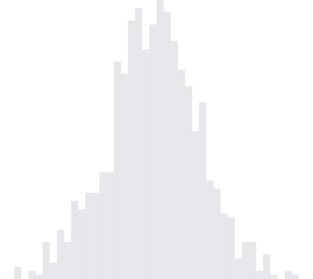
This result might be a little surprising: we start with a scheme that uniformly choose between two uniform distributions, and end up with a stationary distribution that is far from uniform. However, consider that, if $X_{n}$ is already close to one of the edges, then $X_{n + 1}$ has a 50% chance of being even closer to that edge.

Below, we have include code for taking samples from $X_{n}$. Further, we illustrate the convergence of samples from an instance of the $X_{n}$. We notice that the histogram begins to take on the characteristic heavy-tailed shape of the arcsine distribution as the sample size becomes larger and larger.

An instance of samples converging to the arcsine distribution.

next.point <- function(x.prev) {
    u <- runif(1)
    if (u <= 0.5) {
        x.next <- runif(1, 0, x.prev)
    } else {
        x.next <- runif(1, x.prev, 1)
    }
}

sample.n <- function(n, x0 = 0.5) {
    x <- vector(length = n + 1)
    x[1] <- x0
    for (i in 2:(n + 1)) {
        x[i] <- next.point(x[i - 1])
    }
    return(data.frame(x))
}

data <- sample.n(10000)

library(ggplot2)
library(animation)
saveGIF(for (i in 1:500) {
    data.cur = data.frame(data$x[1:(20 * i)])
    colnames(data.cur) <- "x"
    print(ggplot(data.cur) +
        geom_histogram(aes(x = x), binwidth = 0.01) +
        ggtitle(paste(20 * i, "points sampled")))
}, img.name = "samples_plot", outdir = getwd(), interval = 0.15)