Meditations on Mediation

Lately, I’ve been reflecting on how software design could inform statistical methods development. There has always been a two-way flow between methods and applications, and software lies right at the junction. My main thought is that an abstraction originally designed to simplify a computational interface can also guide creative statistical investigation.

I think this is well-illustrated by analyzing the design of the mediation package, so that will be the focus of this post. In the process, we’ll review the basics of mediation analysis and see an illustration using a microbiome-metabolomics dataset.

Mediation Analysis

Mediation analysis is a form of attribution analysis. When we see that a treatment \(T\) influences an outcome \(Y\), we may want to argue that \(T\) influences \(Y\) through a mediator \(M\), represented graphically by:

Here is an alternative visualization. The two colors represent the treatment and the control. \(Y\) depends on both the mediator and the treatment status, represented by the two curves.

If most of the treatment effect can be attributed to the mediator, then it’s a change in the location of the mediators under treatment vs. control that is responsible for change in \(Y\) (left figure). On the other hand, if, for a fixed value of the mediator, we recognize large changes in the response, then the effect of the treatment on the response cannot be attributed to the mediator alone (right figure).

Let’s consider a microbiome example. Intestinal Bowel Disease (IBD) is a condition that can disrupt the lives of its sufferers, and researchers have looked to the microbiome for potential therapies. To better understand how exactly the gut microbial environment differs within IBD patients, the study [Franzosa 2019] gathered both metabolomic (chemical environment) and metagenomic (species abundance) profiles. One thought is that the presence or absence of particular species may mediate changes in the chemical environment for IBD patients. For example, if species \(m\) produces metabolite \(y\), then if we see a decrease in \(y\) among IBD patients, that might be the consequence of species \(m\) being absent. In the notation above, \(T\) is IBD status, the metabolite concentration \(Y\) is the outcome, and the species abundance \(M\) is the mediator.

The most straightforward implementation of mediation analysis assumes the data were drawn from chained linear regressions:

In this notation, the indirect effect that flows through the mediator is computed as \(\alpha \beta_{m}\), while the direct effect which bypasses the mediator is given by \(\beta_{t}\). If we wanted to consider several metabolites and species simultaneously, then we could consider high-dimensional \(M\) and \(Y\) and vector-valued coefficients.

General Mediation Analysis

We could build an interface that encapsulates these chained linear regressions in this way:

mediation <- mediation_analysis(y, m, t)
effects(mediation)

However, we could imagine a more abstract alternative:

f1 <- lm(m ~ t)
f2 <- lm(y ~ t + m)
mediation <- mediation_analysis(f1, f2)
effects(mediation)

The advantage of the second approach is that it could in principle support any mediation or outcome model that the user provides, without our having to implement it internally. For example, in our microbiome application, we could try fitting a logistic-normal mediation model f1 ~ lnm(m ~ t) to account for the ecosystem’s compositional structure.

If we want to use such an interface, though, we will need a new way of computing direct and indirect effects, since we can’t simply read off \(\alpha, \beta_{m}\), and \(\beta_{t}\). Here is where the computational abstraction can inspire a statistical one: We can simulate forward through f1 and f2 to consider a variety of possible outcomes. Specifically, using f1, we can compute \(M\left(t\right)\), the value of the mediator under treatment \(t\). Similarly, using that output from f1, we can also simulate through f2 to generate \(Y\left(M\left(t\right), t'\right)\). Note that we can input different treatment values to f1 and f2 — \(t\) and \(t’\) do not need to be the same.

Given this notation, a new way to define direct and indirect effects is:

Notice that these depend on \(t\), so if we want an overall direct or indirect effect, we could average over \(t = 0, 1\).

Illustration

Let’s work through the microbiome example using this general interface to mediation analysis. The block below reads in and preprocesses the data from the microbiome-metabolome-curated-data repository (a great resource for multi-omics data analysis generated by Elhanan Borenstein’s group at TAU):

Sys.setenv("VROOM_CONNECTION_SIZE" = 5e6)
taxa <- read_tsv("https://raw.githubusercontent.com/borenstein-lab/microbiome-metabolome-curated-data/main/data/processed_data/FRANZOSA_IBD_2019/genera.tsv")[, -1]
metabolites <- read_tsv("https://raw.githubusercontent.com/borenstein-lab/microbiome-metabolome-curated-data/main/data/processed_data/FRANZOSA_IBD_2019/mtb.tsv")[, -1]
metadata <- read_tsv("https://github.com/borenstein-lab/microbiome-metabolome-curated-data/raw/main/data/processed_data/FRANZOSA_IBD_2019/metadata.tsv")

taxa <- clr(taxa) |>
  filter_mean() |>
  simplify_tax_names()

metabolites <- log(1 + metabolites) |>
  filter_mean(threshold = 3) |>
  simplify_metab_names()
  
combined <- metabolites |>
  bind_cols(taxa) |>
  bind_cols(metadata) |>
  mutate(treatment = ifelse(Study.Group == "Control", "control", "treatment"))

The full source code can be found here. So that this process doesn’t take too long, I’ll consider only the twenty most prevalent metabolites and species.

taxa_names <- colnames(taxa)[1:20]
metabolite_names <- colnames(metabolites)[1:20]
mediations <- list()

The glue calls in the block below allow us to define the mediation and outcome models for all pairs of metabolites and taxa under consideration.

pb <- progress_bar$new(total = 400, format = "[:bar] :percent eta: :eta")
for (i in seq_along(metabolite_names)) {
  for (i_prime in seq_along(taxa_names)) {
    fit1 <- lm(formula(glue("{metabolite_names[i]} ~ treatment")), data = combined)
    fit2 <- lm(formula(glue("{metabolite_names[i]} ~ treatment + {taxa_names[i_prime]}")), data = combined)
    pair <- glue("{metabolite_names[i]}_{taxa_names[i_prime]}")
    mediations[[pair]] <- mediate(fit1, fit2, sims = 100, treat = "treatment", mediator = taxa_names[i_prime], control.value = "control", treat.value = "treatment")
    pb$tick()
  }
}

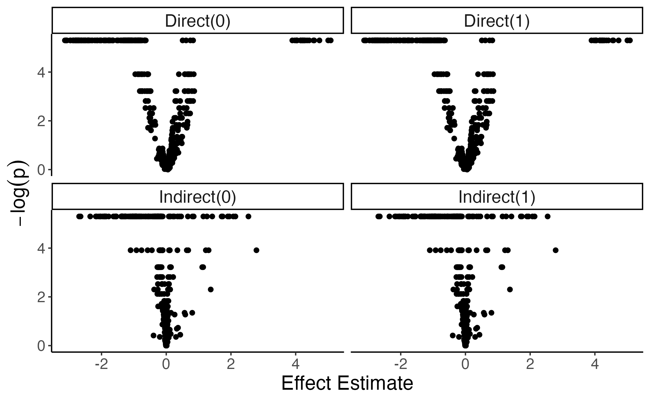
Here is a volcano plot. The package uses a permutation test and occasionally returns \(p\)-values of exactly zero. To ensure that we can still plot \(-log p\), I’ve changed all those exact zeros into¹ \(p = 0.005\). There are direct effects that are clearly both practically and statistically significant, and there even appear to be some promising indirect effects.

Let’s look at these indirect effects more carefully. Here are some of the strongest effects.

> p_values |>
+     filter(term == "Indirect(0)", abs(estimate) > .4, -log(p.value) > 4) |>
+     arrange(-abs(estimate)) |>
+     mutate(across(estimate:p.value, round, 3))
# A tibble: 91 x 6
   metabolite        taxon                 term        estimate std.error p.value
   <chr>             <chr>                 <chr>          <dbl>     <dbl>   <dbl>
 1 C18_eg_Clser_0011 Copromorpha           Indirect(0)    -2.69     0.398   0.005
 2 C18_eg_Clser_0011 Faecousia             Indirect(0)    -2.65     0.396   0.005
 3 C18_eg_Clser_0018 Faecousia             Indirect(0)     2.54     0.687   0.005
 4 C18_eg_Clser_0011 Lachnoclostridium_B   Indirect(0)    -2.35     0.426   0.005
 5 C18_eg_Clser_0011 Marvinbryantia        Indirect(0)    -2.18     0.442   0.005
 6 C18_eg_Clser_0011 Anaeromassilibacillus Indirect(0)    -2.15     0.335   0.005
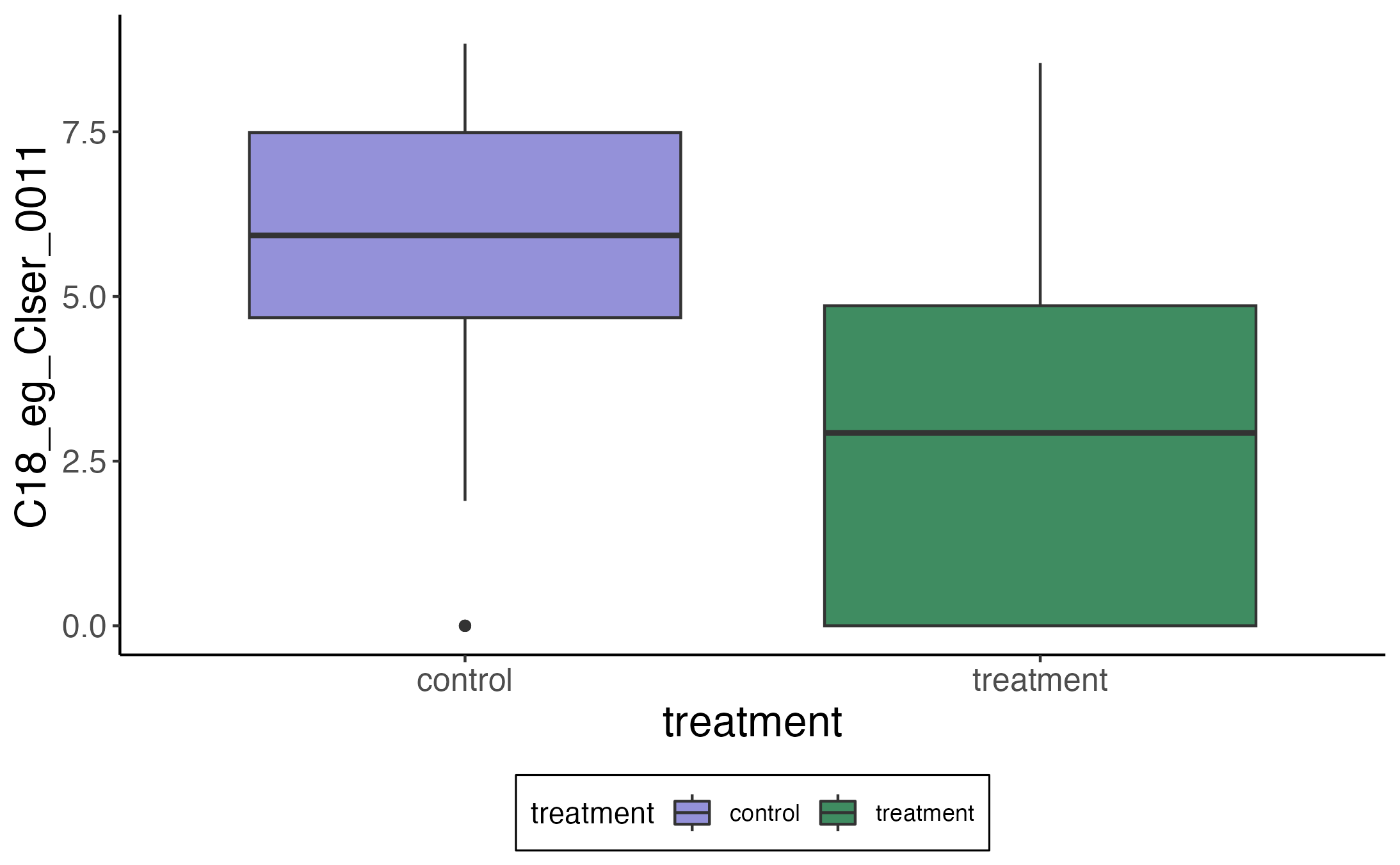
 7 C18_eg_Clser_0018 Lachnoclostridium_B   Indirect(0)     2.14     0.713   0.005

The story for the first row gets a bit complicated, so let’s instead consider the second – how is the metabolite C18_eg_Clser_0011 mediated by the abundance of Faecousia? Here is the difference in the metabolite’s abundance between treatment and control:

And here is the relationship with Faecousia.

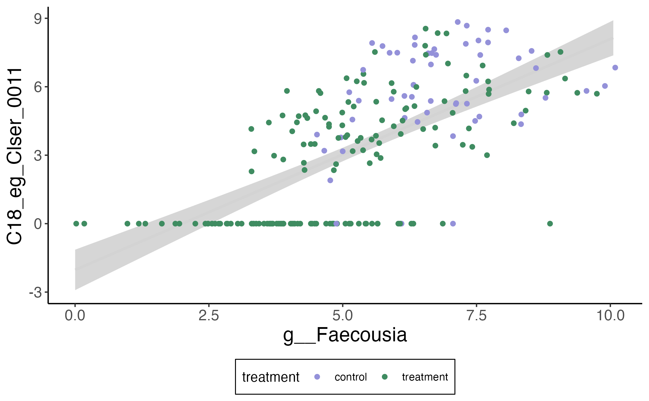
If we ignore the zeros, there does seem to be a clear linear relationship between the metabolite and the abundance of this taxon. Moreover, IBD patients seem to have noticeably fewer of these bacteria relative to the control population. This is nearly a textbook example of an indirect effect — we’re seeing how the change in the mediator result can explain a difference we originally only saw in the outcome.

A few of us in the lab are considering how to make this analysis even more convincing:

1. Instead of filtering so aggressively, ideas from high-dimensional mediation analysis can be used to screen for the most promising pairs of species and metabolites. In this way, we can maintain power while maintaining computational tractability.
2. In this example, a linear outcome model is less satisfying than one that could account for zero inflation. More generally, both the linear and outcome models could include distributions that are commonly used in bioinformatics.

Discussion

An alternative view of this discussion is that software principles can inspire meta-algorithms – there is a direct analogy between functional programming and higher-level statistical algorithms. This is far from a new idea in statistics. For example, when we use boosting or conformal inference, we have to first provide a base learning algorithm as input. Similarly, if we are designing code for use by statistical programmers, it can be valuable to use a functional style, since it makes the code naturally extensible. By letting users freely define a base estimation approach (e.g., the lm calls above), meta-algorithms can have much wider problem-solving reach.

A related point — when I’m creating projects these days, I try to be deliberate about what the interface will look like to the practicing data analyst. This perspective is helpful because it makes me think more carefully about the resulting computational artifacts and how exactly they will look like to the user. For example, the result from plot() or print() should convey clear, qualitative value.