Teaching attention, part 5 / N

The slides are here. Each — marks a new slide.

####

I have this recurring daydream, where I wish I could capture the entire feeling of a moment, without having to try. I feel this sometimes when I walk through a garden, and I try to remember forever exactly how the reflections off the water looked, the patterns of light and shadow on the leaves.

I sometimes feel the same way about data. What if I could understand a raw dataset at a glance? If I were in a competition to identify farmland from satellite imagery, I’d just look the test set and all the coordinates would magically appear in my head.

This unfortunately isn’t possible, but not everything is lost. I mean, we can’t breathe underwater, but we’ve somehow mapped out the ocean floor.

In the same way, people can’t just look at data and make sense of them, but we’ve made a science out of it. It may not be completely effortlesss, but in its own way, I think it’s magical.

In this lecture, we’ll study some of the fundamental ways we can take complex information, and process it in a way so that it makes sense.

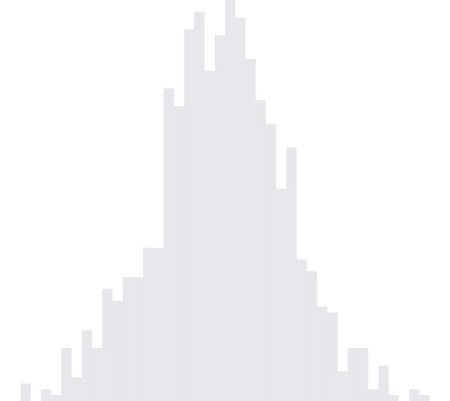
A good mathematical analogy for this process of compressing information is coin flipping. The binomial distribution is a kind of slacker genius, all these outcomes can be flying at it, but it ignores everything except the proportion of outcomes that come up heads. But you can’t blame it, because that’s all you need in order to solve downstream inference tasks.

We need to cary this idea further, this idea that you should capture what is essential, and throw away the rest. Fortunately, there are whole theories built around it. In statistics, it’s called sufficiency, and in deep learning it’s called memory and attention. No matter what you call it, the basic point is the same: good models compress data, whether it’s coin flips into the proportion of heads, or half a terabyte of satellite imagery into a several megabyte neural network.

Next, recurrent neural networks.

RNN cells give a way for computing summaries from streams of information. In a way, they are some of the most fundamental units available for the task. h[t - 1] is our previous summary, then we observe x[t], and based on that new data, we update our summary into h[t]. Visually, the h’s are these blocks, which are continually being updated every time a red input x arrives.

This has a direct analogy to the situation with coin flips. Here, the summaries are estimates of the probability of coming up heads, and the inputs x are the observed coin flips.

Coin flips are nice, but they are discrete. I want to show you an example with continuous data, so let’s consider the related task of counting how many times a time series crosses the interval [0, 1]. It’s similar to counting the number of heads so far, but the raw inputs are no longer binary.

If I move the series around, the summary should update to reflect the new interval counts. (play with the figure)

It turns out that we can completely define a processor that computes this summary, using a two dimensional \(h\). The idea is that to find the number of entrances into the interval, we just need to track whether the series is in the interval at the current timestep, but wasn’t at the previous one. However, our processor can only look at the current input (not the previous one). We can get around this by realizing that we can refer to earlier summaries (we can look at h[t - 1] when finding h[t]), so we’ll just store the previous raw input as the first coordinate of the summary.

This is a mouthful, but the figure below makes it clearer.

I hope you realize how amazing this is. We’ve taken something that’s global, and reduced it to a series of local calculations. This is how memory works. You look at lots of small pieces, one at a time, and combine them into a coherent memory, something that makes sense holistically.

That said, you should be a little disappointed with this approach. We had to handcraft our processors, which goes against the whole philosophy of deep learning. It’s like the picture on the left, we’ve defined some complicated functions during each of the processing steps. They get the job done, but required thought.

Instead, let’s try using the deep learning idea: using compositions of simple functions, plus a little bit of supervision, to automatically learn the best processors. It’s like this picture on the right. We’ll pass the input through many layers, hoping that the combination of simple functions becomes an interesting, complex one.

What should these simple, composable units look like? The answer isn’t too surprising: each layer is a linear function followed by a nonlinearity. The input enters through this term, the previous summary enters through this. For two-dimensional h’s and x’s, we can visualize this directly. The previous summary are the yellow points, and the corresponding update would be the purple h’s. The weight matrices are here in the bottom right. Let’s see what happens when I change the input. (move the input). Does anyone know why it didn’t move anything?

Okay, so those are the units. To learn to compose them in meaningful ways, we need to provide supervision. There are a few different ways we could do this. One approach is to provide a scalar output associated with each sequence. This is like sentiment analysis. The input is a sequence of words in a review, the output is a label for whether the review is positive or negative. An alternative is to supervise each term in the input. This is like in a general language model – your goal might be to predict the next word, given the sequence so far. Finally, your output might itself be a sequence. This is like in Dr. Walcott Brown’s talk, where the input was a medical report, and the output is a sequence of words giving a summary.

In principle, this should be enough for training an RNN. However, as is, these models tend to suffer from something called the vanishing gradient problem. The idea is that since I’m making a small update at every time point, the influence of an early point on the current summary diminishes. The RNN has a memory, but it’s not very long term.

We can also see this visually. Clicking here creates a new input. The new point here is the updated summary. When I create a long sequence of inputs, the units end up saturating, and the summaries collapse. Changing an input early in the sequence has little effect on the summary near the end. This is exactly the vanishing gradient problem – gradients are sensitivity of a value to a perturbation, and if the perturbation leads to very little change, the gradient must be small.

To get around this, and get truly long-term memories, we need to introduce something called gating. These gates keep useful information from getting overwritten. To be honest, I was probably a little sleep deprived when I added this figure, but the point was that these gates are keeping undesirable information from entering.

There are a few different ways to implement gating, but one popular approach are GRUs, gated recurrent units. We introduce variables z[t] and r[t] that control how much the old h and new x can possibly influence the new summary. A large value of z prevents the old summary from contributing much to the new h. A large value of r means that x has somewhat less influence on the new h, compared to the previous h.

This has a nice geometric interpretation, if we go back to the figure. z[t] controls how much h[t] can change between time units. (show this) r[t] controls how much x[t] matters, relative to h[t - 1]. If you set it to 0, it doesn’t matter what the previous h was, it pays attention only to the input value.

With gating, you’ll now be able to train an RNN that learns sophisticated, long-term features. We’re now able to directly learn the counter function that we had hard-coded early on, just by providing lots of examples.

You can see that the model had no idea for the first few epochs, but eventually realizes which points have lots of crossings, and which have none.

We can also inspect the features that were learned. Each row here is one of the h’s, each block is one layer of summaries. You can see that it automatically learned when it’s crossing these bands. The tradeoff is that now you need lots more layers to get the same processor (it’s not just two anymore). So, it’s more automatic, but it’s a bit harded to understand. This is sort of the eternal paradox of deep learning.

Okay, another exercise! Take a few minutes to try this out, work with your neighbor.

That’s everything for gated RNNs. Let’s move on to soft attention. This class of techniques is built of a single observation. We’ve been acting like each new summary h[t] needs to compress the entire past, when in reality, we may be able to refer to summaries we computed before. Our summaries can have structure. And some amount of structure will let us navigate better. Good models do more than just compress information, they compress information in a way that lets us easily navigate it.

We’ll work through this using a canonical application in sequence to sequence modeling: language translation. The goal is to translate a sentence from one to another. I want you to think of this geometrically. Each word is represented by a point in some embedding space, so a sentence is really a sequence of vectors. The sentences in two languages are two sequences in the embedding space. The reason translation is possible is because the sequences will have similar shapes. You basically learn to pattern match different phrases between the languages – the patterns are small subsequences that can be matched between the two languages. Corresponding parts of the h space have similar meanings.

So, from the most abstract point of view, we are learning to transform one sequence to another which has a similar shape.

Now, to tackle the translation problem, we can make use of a slight variant of gated RNNs. We take the original sequence, and encode them into a sequence of summaries h. The last summary h is supposed to capture the entire shape of the source sentence. We use that to initialize a decoder, which builds a new sequence of summaries (these blue ones). The point is that, if your meaning is currently \tilde{h}[t - 1], and your previous word was y[t - 1], then a good guess for the meaning of the next word is tilde{h}[t]. From the meaning’s \tilde{h}[t], you should be able to predict a most plausible y[t]. Unlike usual gated RNNs, you also are allowed to look at this last summary h[T], at any timepoint you want.

A word of caution. You never see the real y[t - 1]. If you could, you wouldn’t need to do the translation task in the first place. So when I said you take y[t - 1] as input, I lied. You would usually make a prediction of the word y[t] at each step, based on the current \tilde{h}[t], and use that predicted sequence as if it were the truth. The distance between the decoded and true sequences is basically the error of your translation model.

Now, where does attention fit in? The point is that it’s a huge burden on this last summary, to have to memorize the entire sequence. It’s helped that we use gating, but it’s not enough. Instead, it’s reasonable to think that, to identify the meaning for some word near the beginning of the target sentence, it’s enough to pay attention solely to the summaries near the start of the source sentence. This is because the meanings are usually similar, between the parts of the sentence.

Concretely, at the t^th decoding step, we now are allowed to look at some weighted combination of the source encodings. The weights should be highest on parts of the source sentence that are most similar in meaning to the part that we are currently trying to decode.

When I move along the sentence, I should change the weight distribution.

This sounds useful, but how do we actually find the weights \alpha? Two approaches are really common. The first, location based attention, matches similar points if they occur in similar points in the sentence. The second, content based attention, looks for similarities in meaning. That’s what I’m trying to say in this figure. Location based has high weight around the decoding position. Content based attention puts high weight on these points though (near the end of the sentence), because, even though they are far in terms of sequence position, they have similar meanings (remember, location in the embedding space corresponds to meaning).

Mathematically, these are computed using these different softmaxes. The first softmax doesn’t look at the values of the summaries h[t], it doesn’t need to refer to content. They’re both linear combinations of the current decoding h, but only the second looks at the earlier encodings.

Okay, another exercise! Take a few minutes to try this out, work with your neighbor.

The final big idea of this part of the lecture: hard attention. Sometimes we have a huge dataset, but only a tiny part is really relevant for the tasks we have in mind. Is there any way we can avoid doing all this unecessary computation? For example, let’s say we wanted to figure out what the speed limit is, from this image. We should learn to attend to this tiny part of the image, and ignore everything else.

Our approach will be to crop the image into a few relevant pieces, make a good summary of these pieces, and then use them to classify.

Let’s address each of these components, one at a time. Suppose we knew where to crop, the idea is to extract a few windows around the crop location, at different zoom levels. Then, along with the proposed location, we encode everything into g[t]. The encodings are actually really straightforwards, they’re just MLPs.

Once we have these encodings, how will we classify? This picture should remind you a lot of the earlier part of this talk…

We can use an RNN. We treat the sequence of encoded crops as a sequence of inputs to an RNN. The orange rectangles are now a sequence of summaries, just like the coin flipping summaries from before. The last of these summaries should have a memory of all the encodings we’ve seen so far. This is what we’ll use for the final classification.

There is this lingering issue of where to define the cropping locations. But the RNN perspective basically solves this problem. We can use the latest summary ot predict the next crop location. This should make sure that we crop out important locations that we haven’t looked at before.

We’re sooo close, but it’s still not enough. The approach works better if you have some randomness in where you look. It makes some sense – you don’t want your previous crops to completely predetermine your next proposal. Instead, they sample the crops around some mean, and the mean is a function of the previous summary states. Conceptually, this is nice, but it introduces some difficulties with training. We can’t just backpropagate everything.

More precisely, we want to propose a mean cropping location in such a way that, across many random samples around that location, these classification errors are small. This is different from the usual neural network objective, where we’re trying to minimize a deterministic loss, which depends on the network parameters.

Fortunately, there is work on how you do this. I could just show you some math, but I think it’s better if we look at some plots.

A refresher, how does gradient descent work? You need to be able to evaluate the loss at the current parameter \(\mu\). Then, you move your parameter in the negative gradient direction.

The only problem with using gradient descent now is that… we see neither \(f\left(\mu\right)\)… nor it’s gradient. So, we flat out just can’t do gradient descent. We observe these red points, which are random crops around the deterministic mean. How should we update our parameter? Well, if you look at this plot, it makes sense to move it in a direction where the f’s typically seem pretty small.

It turns out that this is exactly what this mathematical identity tells you to do. To take the gradient of this expectation, you can average over a weighted score function. These terms are directions, relative to the current parameter value. The weights are higher for points that have higher values of f. If all the f’s were comparable, then this is basically 0, since the locations have mean

But if some of the f’s are much larger than others, we’ll move in those directions. (well really, we move in the negative gradient direction, since we’re trying to minimize the function).

Here’s an interactive illustration of that idea. It takes some time, but eventually it learns to put the mean near the the bottom of this function.

At this point, you have everything you need to implement a recurrent hard attention model. You have modules for cropping images and making predictions, and you know a way to optimize functions that have an element of randomness.

And that wraps up part 1. There were three major topics: gating, soft attention, and hard attention. Gating made sure that inputs from early on could still influence summaries at a later point, making meaningful compression possible across long sequences. Soft attention let us navigate a larger collection of local summaries. And hard attention allowed us to focus on just the parts of the input that matters, reducing a lot of the computational burden.

In the second part, we’ll discuss more sophisticated approaches modules for building these summaries. With that, thank you, and take it away Aidan!